

Appendix F.1: Non-paralyzable
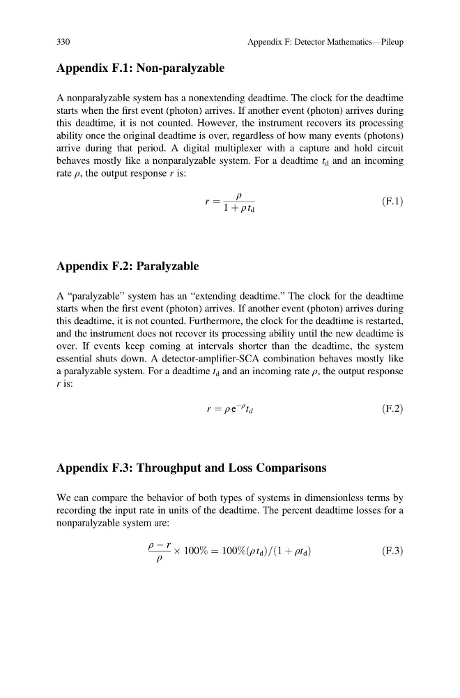
A nonparalyzable system has a nonextending deadtime. The clock for the deadtime
starts when the first event (photon) arrives. If another event (photon) arrives during
this deadtime, it is not counted. However, the instrument recovers its processing
ability once the original deadtime is over, regardless of how many events (photons)
arrive during that period. A digital multiplexer with a capture and hold circuit
behaves mostly like a nonparalyzable system. For a deadtime t d and an incoming
rate ρ, the output response r is:
r ¼
ρ
1 þ ρ t d
ðF:1Þ
Appendix F.2: Paralyzable
A “paralyzable” system has an “extending deadtime.” The clock for the deadtime
starts when the first event (photon) arrives. If another event (photon) arrives during
this deadtime, it is not counted. Furthermore, the clock for the deadtime is restarted,
and the instrument does not recover its processing ability until the new deadtime is
over. If events keep coming at intervals shorter than the deadtime, the system
essential shuts down. A detector-amplifier-SCA combination behaves mostly like
a paralyzable system. For a deadtime t d and an incoming rate ρ, the output response
r is:
r ¼ ρ e
Àρ t d
ðF:2Þ
Appendix F.3: Throughput and Loss Comparisons
We can compare the behavior of both types of systems in dimensionless terms by
recording the input rate in units of the deadtime. The percent deadtime losses for a
nonparalyzable system are:
ρ À r
ρ
 100% ¼ 100% ρ t d
ð Þ= 1 þ ρt d
ð
Þ
ðF:3Þ
330
Appendix F: Detector Mathematics—Pileup
A nonparalyzable system has a nonextending deadtime. The clock for the deadtime
starts when the first event (photon) arrives. If another event (photon) arrives during
this deadtime, it is not counted. However, the instrument recovers its processing
ability once the original deadtime is over, regardless of how many events (photons)
arrive during that period. A digital multiplexer with a capture and hold circuit
behaves mostly like a nonparalyzable system. For a deadtime t d and an incoming
rate ρ, the output response r is:
r ¼
ρ
1 þ ρ t d
ðF:1Þ
Appendix F.2: Paralyzable
A “paralyzable” system has an “extending deadtime.” The clock for the deadtime
starts when the first event (photon) arrives. If another event (photon) arrives during
this deadtime, it is not counted. Furthermore, the clock for the deadtime is restarted,
and the instrument does not recover its processing ability until the new deadtime is
over. If events keep coming at intervals shorter than the deadtime, the system
essential shuts down. A detector-amplifier-SCA combination behaves mostly like
a paralyzable system. For a deadtime t d and an incoming rate ρ, the output response
r is:
r ¼ ρ e
Àρ t d
ðF:2Þ
Appendix F.3: Throughput and Loss Comparisons
We can compare the behavior of both types of systems in dimensionless terms by
recording the input rate in units of the deadtime. The percent deadtime losses for a
nonparalyzable system are:
ρ À r
ρ
 100% ¼ 100% ρ t d
ð Þ= 1 þ ρt d
ð
Þ
ðF:3Þ
330
Appendix F: Detector Mathematics—Pileup