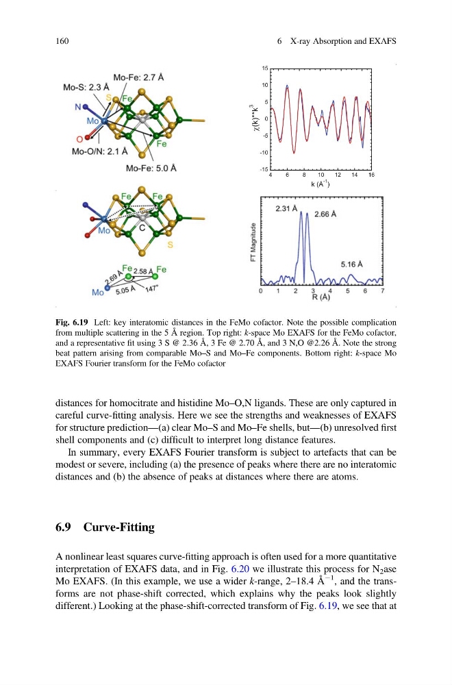
distances for homocitrate and histidine Mo–O,N ligands. These are only captured in
careful curve-fitting analysis. Here we see the strengths and weaknesses of EXAFS
for structure prediction—(a) clear Mo–S and Mo–Fe shells, but—(b) unresolved first
shell components and (c) difficult to interpret long distance features.
In summary, every EXAFS Fourier transform is subject to artefacts that can be
modest or severe, including (a) the presence of peaks where there are no interatomic
distances and (b) the absence of peaks at distances where there are atoms.
6.9 Curve-Fitting
A nonlinear least squares curve-fitting approach is often used for a more quantitative
interpretation of EXAFS data, and in Fig. 6.20 we illustrate this process for N 2 ase
Mo EXAFS. (In this example, we use a wider k-range, 2–18.4 Å
À1 , and the transforms are not phase-shift corrected, which explains why the peaks look slightly
different.) Looking at the phase-shift-corrected transform of Fig. 6.19, we see that at
-15
-10
-5
0
5
10
15
4
6
8
1 0
1 2
1 4
1 6
k (Å
-1 )
c(k)**k
3
Fig. 6.19 Left: key interatomic distances in the FeMo cofactor. Note the possible complication
from multiple scattering in the 5 Å region. Top right: k-space Mo EXAFS for the FeMo cofactor,
and a representative fit using 3 S @ 2.36 Å, 3 Fe @ 2.70 Å, and 3 N,O @2.26 Å. Note the strong
beat pattern arising from comparable Mo–S and Mo–Fe components. Bottom right: k-space Mo
EXAFS Fourier transform for the FeMo cofactor
160
6 X-ray Absorption and EXAFS