

1 The Potential Energy Surface in Molecular Quantum Mechanics
35
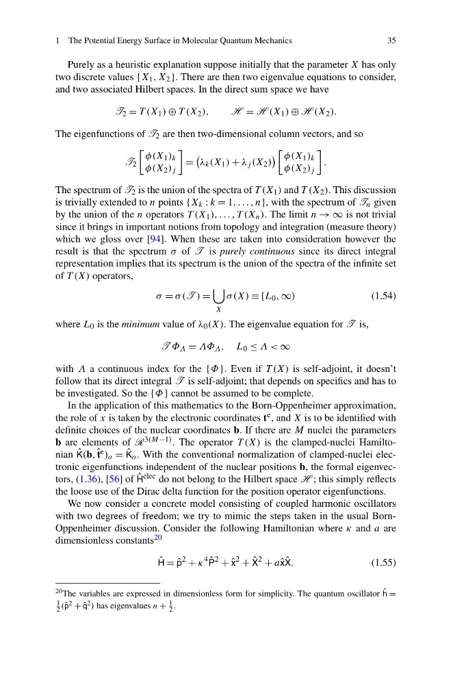
Purely as a heuristic explanation suppose initially that the parameter X has only
two discrete values {X 1 , X 2 }. There are then two eigenvalue equations to consider,
and two associated Hilbert spaces. In the direct sum space we have
T 2 = T (X 1 ) ⊕ T (X 2 ),
H = H (X 1 ) ⊕ H (X 2 ).
The eigenfunctions of T 2 are then two-dimensional column vectors, and so
T 2
φ(X 1 ) k
φ(X 2 ) j
=
λ k (X 1 ) + λ j (X 2 )
φ(X 1 ) k
φ(X 2 ) j
.
The spectrum of T 2 is the union of the spectra of T (X 1 ) and T (X 2 ). This discussion
is trivially extended to n points {X k : k = 1, . . . , n}, with the spectrum of T n given
by the union of the n operators T (X 1 ), . . . , T (X n ). The limit n → ∞ is not trivial
since it brings in important notions from topology and integration (measure theory)
which we gloss over [94]. When these are taken into consideration however the
result is that the spectrum σ of T is purely continuous since its direct integral
representation implies that its spectrum is the union of the spectra of the infinite set
of T (X) operators,
σ = σ (T ) =
X
σ (X) ≡ [L 0 , ∞)
(1.54)
where L 0 is the minimum value of λ 0 (X). The eigenvalue equation for T is,
T Φ Λ = ΛΦ Λ , L 0 ≤ Λ < ∞
with Λ a continuous index for the {Φ}. Even if T (X) is self-adjoint, it doesn’t
follow that its direct integral T is self-adjoint; that depends on specifics and has to
be investigated. So the {Φ} cannot be assumed to be complete.
In the application of this mathematics to the Born-Oppenheimer approximation,
the role of x is taken by the electronic coordinates t e , and X is to be identified with
definite choices of the nuclear coordinates b. If there are M nuclei the parameters
b are elements of R 3(M−1) . The operator T (X) is the clamped-nuclei Hamiltonian ˆ
K(b, ˆ t e ) o = ˆ
K o . With the conventional normalization of clamped-nuclei electronic eigenfunctions independent of the nuclear positions b, the formal eigenvectors, (1.36), [56] of ˆ
H elec do not belong to the Hilbert space H ; this simply reflects
the loose use of the Dirac delta function for the position operator eigenfunctions.
We now consider a concrete model consisting of coupled harmonic oscillators
with two degrees of freedom; we try to mimic the steps taken in the usual BornOppenheimer discussion. Consider the following Hamiltonian where κ and a are
dimensionless constants 20
ˆ
H = ˆ
p
2
+ κ
4 ˆ
P
2
+ ˆ
x
2
+ ˆ
X
2
+ a ˆ
x ˆ
X.
(1.55)
20 The variables are expressed in dimensionless form for simplicity. The quantum oscillator ˆ
h =
1
2 (ˆ p 2 + ˆ
q 2 ) has eigenvalues n +
1
2 .
35
Purely as a heuristic explanation suppose initially that the parameter X has only
two discrete values {X 1 , X 2 }. There are then two eigenvalue equations to consider,
and two associated Hilbert spaces. In the direct sum space we have
T 2 = T (X 1 ) ⊕ T (X 2 ),
H = H (X 1 ) ⊕ H (X 2 ).
The eigenfunctions of T 2 are then two-dimensional column vectors, and so
T 2
φ(X 1 ) k
φ(X 2 ) j
=
λ k (X 1 ) + λ j (X 2 )
φ(X 1 ) k
φ(X 2 ) j
.
The spectrum of T 2 is the union of the spectra of T (X 1 ) and T (X 2 ). This discussion
is trivially extended to n points {X k : k = 1, . . . , n}, with the spectrum of T n given
by the union of the n operators T (X 1 ), . . . , T (X n ). The limit n → ∞ is not trivial
since it brings in important notions from topology and integration (measure theory)
which we gloss over [94]. When these are taken into consideration however the
result is that the spectrum σ of T is purely continuous since its direct integral
representation implies that its spectrum is the union of the spectra of the infinite set
of T (X) operators,
σ = σ (T ) =
X
σ (X) ≡ [L 0 , ∞)
(1.54)
where L 0 is the minimum value of λ 0 (X). The eigenvalue equation for T is,
T Φ Λ = ΛΦ Λ , L 0 ≤ Λ < ∞
with Λ a continuous index for the {Φ}. Even if T (X) is self-adjoint, it doesn’t
follow that its direct integral T is self-adjoint; that depends on specifics and has to
be investigated. So the {Φ} cannot be assumed to be complete.
In the application of this mathematics to the Born-Oppenheimer approximation,
the role of x is taken by the electronic coordinates t e , and X is to be identified with
definite choices of the nuclear coordinates b. If there are M nuclei the parameters
b are elements of R 3(M−1) . The operator T (X) is the clamped-nuclei Hamiltonian ˆ
K(b, ˆ t e ) o = ˆ
K o . With the conventional normalization of clamped-nuclei electronic eigenfunctions independent of the nuclear positions b, the formal eigenvectors, (1.36), [56] of ˆ
H elec do not belong to the Hilbert space H ; this simply reflects
the loose use of the Dirac delta function for the position operator eigenfunctions.
We now consider a concrete model consisting of coupled harmonic oscillators
with two degrees of freedom; we try to mimic the steps taken in the usual BornOppenheimer discussion. Consider the following Hamiltonian where κ and a are
dimensionless constants 20
ˆ
H = ˆ
p
2
+ κ
4 ˆ
P
2
+ ˆ
x
2
+ ˆ
X
2
+ a ˆ
x ˆ
X.
(1.55)
20 The variables are expressed in dimensionless form for simplicity. The quantum oscillator ˆ
h =
1
2 (ˆ p 2 + ˆ
q 2 ) has eigenvalues n +
1
2 .