

15 Molecular Theory of Graphene
263
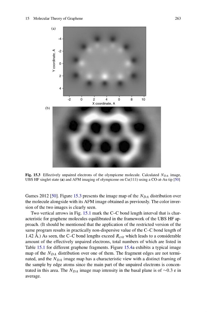
Fig. 15.3 Effectively unpaired electrons of the olympicene molecule. Calculated N DA image,
UBS HF singlet state (a) and AFM imaging of olympicene on Cu(111) using a CO-at-Au tip [50]
Games 2012 [50]. Figure 15.3 presents the image map of the N DA distribution over
the molecule alongside with its AFM image obtained as previously. The color inversion of the two images is clearly seen.
Two vertical arrows in Fig. 15.1 mark the C–C bond length interval that is characteristic for graphene molecules equilibrated in the framework of the UBS HF approach. (It should be mentioned that the application of the restricted version of the
same program results in practically non-dispersive value of the C–C bond length of
1.42 Å.) As seen, the C–C bond lengths exceed R crit which leads to a considerable
amount of the effectively unpaired electrons, total numbers of which are listed in
Table 15.1 for different graphene fragments. Figure 15.4a exhibits a typical image
map of the N DA distribution over one of them. The fragment edges are not terminated, and the N DA image map has a characteristic view with a distinct framing of
the sample by edge atoms since the main part of the unpaired electrons is concentrated in this area. The N DA image map intensity in the basal plane is of ∼0.3 e in
average.
263
Fig. 15.3 Effectively unpaired electrons of the olympicene molecule. Calculated N DA image,
UBS HF singlet state (a) and AFM imaging of olympicene on Cu(111) using a CO-at-Au tip [50]
Games 2012 [50]. Figure 15.3 presents the image map of the N DA distribution over
the molecule alongside with its AFM image obtained as previously. The color inversion of the two images is clearly seen.
Two vertical arrows in Fig. 15.1 mark the C–C bond length interval that is characteristic for graphene molecules equilibrated in the framework of the UBS HF approach. (It should be mentioned that the application of the restricted version of the
same program results in practically non-dispersive value of the C–C bond length of
1.42 Å.) As seen, the C–C bond lengths exceed R crit which leads to a considerable
amount of the effectively unpaired electrons, total numbers of which are listed in
Table 15.1 for different graphene fragments. Figure 15.4a exhibits a typical image
map of the N DA distribution over one of them. The fragment edges are not terminated, and the N DA image map has a characteristic view with a distinct framing of
the sample by edge atoms since the main part of the unpaired electrons is concentrated in this area. The N DA image map intensity in the basal plane is of ∼0.3 e in
average.