

5 Application of the Uniformly Charged Sphere Stabilization
107
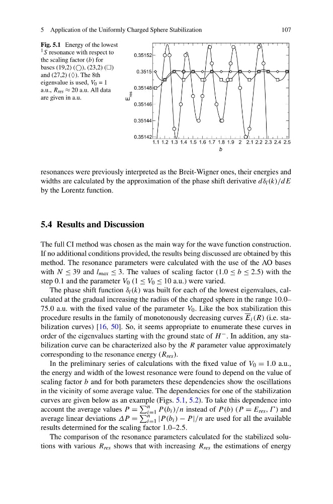
Fig. 5.1 Energy of the lowest
1 S resonance with respect to
the scaling factor (b) for
bases (19,2) (), (23,2) ()
and (27,2) (♦). The 8th
eigenvalue is used, V 0 = 1
a.u., R res ≈ 20 a.u. All data
are given in a.u.
resonances were previously interpreted as the Breit-Wigner ones, their energies and
widths are calculated by the approximation of the phase shift derivative dδ l (k)/dE
by the Lorentz function.
5.4 Results and Discussion
The full CI method was chosen as the main way for the wave function construction.
If no additional conditions provided, the results being discussed are obtained by this
method. The resonance parameters were calculated with the use of the AO bases
with N ≤ 39 and l max ≤ 3. The values of scaling factor (1.0 ≤ b ≤ 2.5) with the
step 0.1 and the parameter V 0 (1 ≤ V 0 ≤ 10 a.u.) were varied.
The phase shift function δ l (k) was built for each of the lowest eigenvalues, calculated at the gradual increasing the radius of the charged sphere in the range 10.0–
75.0 a.u. with the fixed value of the parameter V 0 . Like the box stabilization this
procedure results in the family of monotonously decreasing curves E i (R) (i.e. stabilization curves) [16, 50]. So, it seems appropriate to enumerate these curves in
order of the eigenvalues starting with the ground state of H − . In addition, any stabilization curve can be characterized also by the R parameter value approximately
corresponding to the resonance energy (R res ).
In the preliminary series of calculations with the fixed value of V 0 = 1.0 a.u.,
the energy and width of the lowest resonance were found to depend on the value of
scaling factor b and for both parameters these dependencies show the oscillations
in the vicinity of some average value. The dependencies for one of the stabilization
curves are given below as an example (Figs. 5.1, 5.2). To take this dependence into
account the average values P =
n
i=1 P (b i )/n instead of P (b) (P = E res , Γ ) and
average linear deviations ΔP =
n
i=1 |P (b i ) − P |/n are used for all the available
results determined for the scaling factor 1.0–2.5.
The comparison of the resonance parameters calculated for the stabilized solutions with various R res shows that with increasing R res the estimations of energy
107
Fig. 5.1 Energy of the lowest
1 S resonance with respect to
the scaling factor (b) for
bases (19,2) (), (23,2) ()
and (27,2) (♦). The 8th
eigenvalue is used, V 0 = 1
a.u., R res ≈ 20 a.u. All data
are given in a.u.
resonances were previously interpreted as the Breit-Wigner ones, their energies and
widths are calculated by the approximation of the phase shift derivative dδ l (k)/dE
by the Lorentz function.
5.4 Results and Discussion
The full CI method was chosen as the main way for the wave function construction.
If no additional conditions provided, the results being discussed are obtained by this
method. The resonance parameters were calculated with the use of the AO bases
with N ≤ 39 and l max ≤ 3. The values of scaling factor (1.0 ≤ b ≤ 2.5) with the
step 0.1 and the parameter V 0 (1 ≤ V 0 ≤ 10 a.u.) were varied.
The phase shift function δ l (k) was built for each of the lowest eigenvalues, calculated at the gradual increasing the radius of the charged sphere in the range 10.0–
75.0 a.u. with the fixed value of the parameter V 0 . Like the box stabilization this
procedure results in the family of monotonously decreasing curves E i (R) (i.e. stabilization curves) [16, 50]. So, it seems appropriate to enumerate these curves in
order of the eigenvalues starting with the ground state of H − . In addition, any stabilization curve can be characterized also by the R parameter value approximately
corresponding to the resonance energy (R res ).
In the preliminary series of calculations with the fixed value of V 0 = 1.0 a.u.,
the energy and width of the lowest resonance were found to depend on the value of
scaling factor b and for both parameters these dependencies show the oscillations
in the vicinity of some average value. The dependencies for one of the stabilization
curves are given below as an example (Figs. 5.1, 5.2). To take this dependence into
account the average values P =
n
i=1 P (b i )/n instead of P (b) (P = E res , Γ ) and
average linear deviations ΔP =
n
i=1 |P (b i ) − P |/n are used for all the available
results determined for the scaling factor 1.0–2.5.
The comparison of the resonance parameters calculated for the stabilized solutions with various R res shows that with increasing R res the estimations of energy