

94
E.J. Brändas
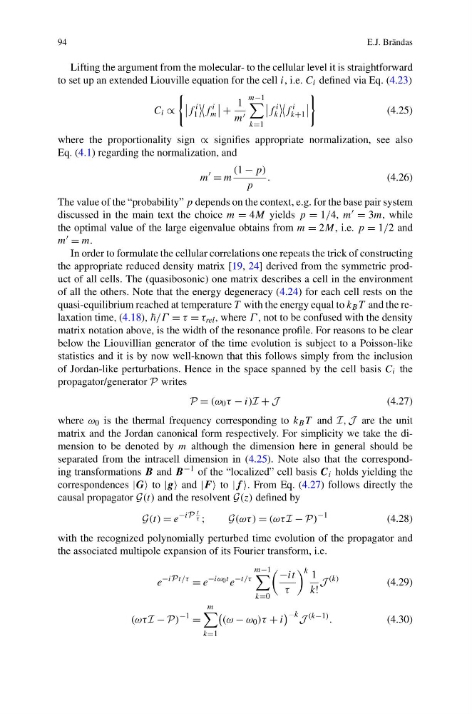
Lifting the argument from the molecular- to the cellular level it is straightforward
to set up an extended Liouville equation for the cell i, i.e. C i defined via Eq. (4.23)
C i ∝
f
i
1
f
i
m
+
1
m
m−1
k=1
f
i
k
f
i
k+1
(4.25)
where the proportionality sign ∝ signifies appropriate normalization, see also
Eq. (4.1) regarding the normalization, and
m
= m
(1 − p)
p
.
(4.26)
The value of the “probability” p depends on the context, e.g. for the base pair system
discussed in the main text the choice m = 4M yields p = 1/4, m = 3m, while
the optimal value of the large eigenvalue obtains from m = 2M, i.e. p = 1/2 and
m = m.
In order to formulate the cellular correlations one repeats the trick of constructing
the appropriate reduced density matrix [19, 24] derived from the symmetric product of all cells. The (quasibosonic) one matrix describes a cell in the environment
of all the others. Note that the energy degeneracy (4.24) for each cell rests on the
quasi-equilibrium reached at temperature T with the energy equal to k B T and the relaxation time, (4.18), /Γ = τ = τ rel , where Γ , not to be confused with the density
matrix notation above, is the width of the resonance profile. For reasons to be clear
below the Liouvillian generator of the time evolution is subject to a Poisson-like
statistics and it is by now well-known that this follows simply from the inclusion
of Jordan-like perturbations. Hence in the space spanned by the cell basis C i the
propagator/generator P writes
P = (ω 0 τ − i)I + J
(4.27)
where ω 0 is the thermal frequency corresponding to k B T and I, J are the unit
matrix and the Jordan canonical form respectively. For simplicity we take the dimension to be denoted by m although the dimension here in general should be
separated from the intracell dimension in (4.25). Note also that the corresponding transformations B and B −1 of the “localized” cell basis C i holds yielding the
correspondences |G to |g and |F to |f . From Eq. (4.27) follows directly the
causal propagator G(t) and the resolvent G(z) defined by
G(t) = e
−iP
t
τ ;
G(ωτ ) = (ωτ I − P)
−1
(4.28)
with the recognized polynomially perturbed time evolution of the propagator and
the associated multipole expansion of its Fourier transform, i.e.
e
−iPt/τ
= e
−iω 0 t e
−t/τ
m−1
k=0
−it
τ
k 1
k!
J
(k)
(4.29)
(ωτ I − P)
−1
=
m
k=1
(ω − ω 0 )τ + i
−k J
(k−1) .
(4.30)
E.J. Brändas
Lifting the argument from the molecular- to the cellular level it is straightforward
to set up an extended Liouville equation for the cell i, i.e. C i defined via Eq. (4.23)
C i ∝
f
i
1
f
i
m
+
1
m
m−1
k=1
f
i
k
f
i
k+1
(4.25)
where the proportionality sign ∝ signifies appropriate normalization, see also
Eq. (4.1) regarding the normalization, and
m
= m
(1 − p)
p
.
(4.26)
The value of the “probability” p depends on the context, e.g. for the base pair system
discussed in the main text the choice m = 4M yields p = 1/4, m = 3m, while
the optimal value of the large eigenvalue obtains from m = 2M, i.e. p = 1/2 and
m = m.
In order to formulate the cellular correlations one repeats the trick of constructing
the appropriate reduced density matrix [19, 24] derived from the symmetric product of all cells. The (quasibosonic) one matrix describes a cell in the environment
of all the others. Note that the energy degeneracy (4.24) for each cell rests on the
quasi-equilibrium reached at temperature T with the energy equal to k B T and the relaxation time, (4.18), /Γ = τ = τ rel , where Γ , not to be confused with the density
matrix notation above, is the width of the resonance profile. For reasons to be clear
below the Liouvillian generator of the time evolution is subject to a Poisson-like
statistics and it is by now well-known that this follows simply from the inclusion
of Jordan-like perturbations. Hence in the space spanned by the cell basis C i the
propagator/generator P writes
P = (ω 0 τ − i)I + J
(4.27)
where ω 0 is the thermal frequency corresponding to k B T and I, J are the unit
matrix and the Jordan canonical form respectively. For simplicity we take the dimension to be denoted by m although the dimension here in general should be
separated from the intracell dimension in (4.25). Note also that the corresponding transformations B and B −1 of the “localized” cell basis C i holds yielding the
correspondences |G to |g and |F to |f . From Eq. (4.27) follows directly the
causal propagator G(t) and the resolvent G(z) defined by
G(t) = e
−iP
t
τ ;
G(ωτ ) = (ωτ I − P)
−1
(4.28)
with the recognized polynomially perturbed time evolution of the propagator and
the associated multipole expansion of its Fourier transform, i.e.
e
−iPt/τ
= e
−iω 0 t e
−t/τ
m−1
k=0
−it
τ
k 1
k!
J
(k)
(4.29)
(ωτ I − P)
−1
=
m
k=1
(ω − ω 0 )τ + i
−k J
(k−1) .
(4.30)