

4.2 Development of a Mathematical Model
69
Y = bacteria yield coefficient,
b s = biomass loss rate due to shearing from biofilm, day
−1 ,
b t = total biomass loss rate from biofilm, day
−1 ,
b d = biomass decay coefficient, day
−1 ,
θ c = mean cell residence time or solid retention time (day).
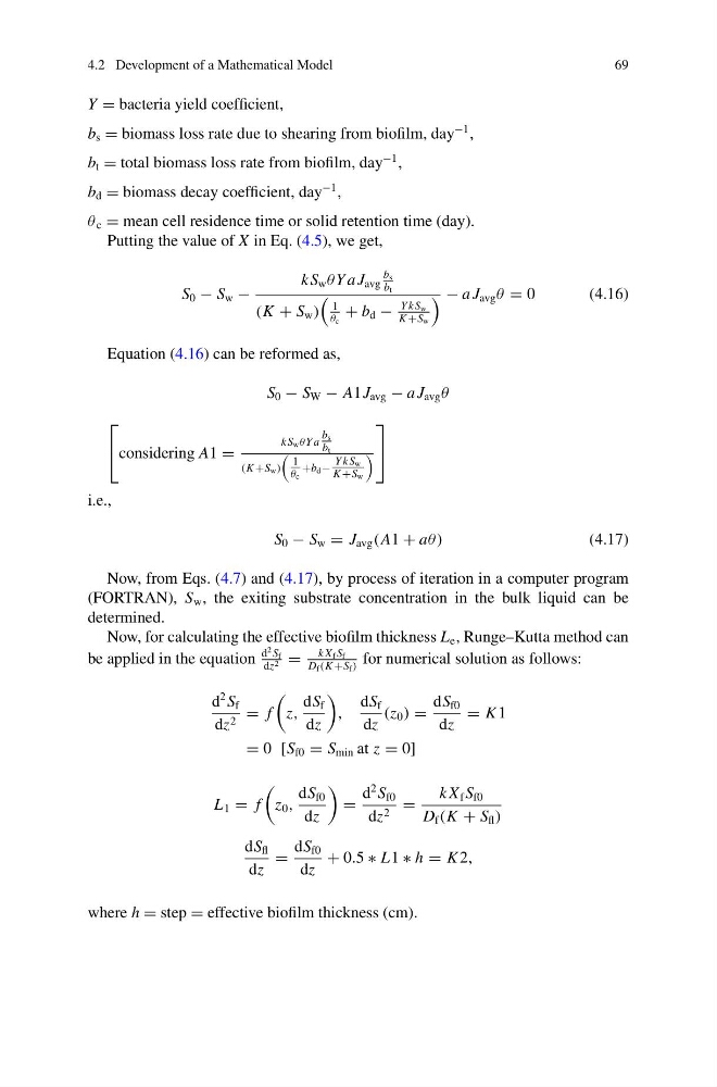
Putting the value of X in Eq. (4.5), we get,
S 0 − S w −
kS w θ Y a J avg
b s
b t
(K + S w )
1
θ c
+ b d −
Y kS w
K +S w
− a J avg θ = 0
(4.16)
Equation (4.16) can be reformed as,
S 0 − S W − A1J avg − a J avg θ
⎡
⎣ considering A1 =
kS w θ Y a
b s
b t
(K +S w )
1
θ c
+b d −
Y kS w
K +S w
⎤
⎦
i.e.,
S 0 − S w = J avg (A1 + aθ)
(4.17)
Now, from Eqs. (4.7) and (4.17), by process of iteration in a computer program
(FORTRAN), S w , the exiting substrate concentration in the bulk liquid can be
determined.
Now, for calculating the effective biofilm thickness L e , Runge–Kutta method can
be applied in the equation
d
2 S f
dz 2 =
k X f S f
D f (K +S f )
for numerical solution as follows:
d
2 S f
dz 2 = f
z,
dS f
dz
,
dS f
dz
(z 0 ) =
dS f0
dz
= K 1
= 0 [S f0 = S min at z = 0]
L 1 = f
z 0 ,
dS f0
dz
=
d
2 S f0
dz 2 =
k X f S f0
D f (K + S fl )
dS fl
dz
=
dS f0
dz
+ 0.5 ∗ L1 ∗ h = K 2,
where h = step = effective biofilm thickness (cm).
69
Y = bacteria yield coefficient,
b s = biomass loss rate due to shearing from biofilm, day
−1 ,
b t = total biomass loss rate from biofilm, day
−1 ,
b d = biomass decay coefficient, day
−1 ,
θ c = mean cell residence time or solid retention time (day).
Putting the value of X in Eq. (4.5), we get,
S 0 − S w −
kS w θ Y a J avg
b s
b t
(K + S w )
1
θ c
+ b d −
Y kS w
K +S w
− a J avg θ = 0
(4.16)
Equation (4.16) can be reformed as,
S 0 − S W − A1J avg − a J avg θ
⎡
⎣ considering A1 =
kS w θ Y a
b s
b t
(K +S w )
1
θ c
+b d −
Y kS w
K +S w
⎤
⎦
i.e.,
S 0 − S w = J avg (A1 + aθ)
(4.17)
Now, from Eqs. (4.7) and (4.17), by process of iteration in a computer program
(FORTRAN), S w , the exiting substrate concentration in the bulk liquid can be
determined.
Now, for calculating the effective biofilm thickness L e , Runge–Kutta method can
be applied in the equation
d
2 S f
dz 2 =
k X f S f
D f (K +S f )
for numerical solution as follows:
d
2 S f
dz 2 = f
z,
dS f
dz
,
dS f
dz
(z 0 ) =
dS f0
dz
= K 1
= 0 [S f0 = S min at z = 0]
L 1 = f
z 0 ,
dS f0
dz
=
d
2 S f0
dz 2 =
k X f S f0
D f (K + S fl )
dS fl
dz
=
dS f0
dz
+ 0.5 ∗ L1 ∗ h = K 2,
where h = step = effective biofilm thickness (cm).