

190
K. A. S. Fessler et al.
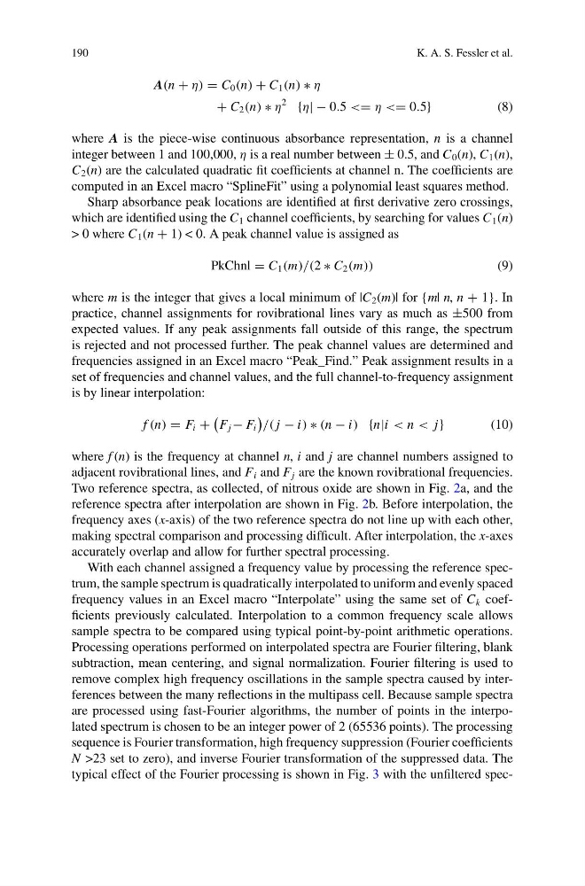
A(n + η) = C 0 (n) + C 1 (n) ∗ η
+ C 2 (n) ∗ η
2
{η| − 0.5 <= η <= 0.5}
(8)
where A is the piece-wise continuous absorbance representation, n is a channel
integer between 1 and 100,000, η is a real number between ± 0.5, and C 0 (n), C 1 (n),
C 2 (n) are the calculated quadratic fit coefficients at channel n. The coefficients are
computed in an Excel macro “SplineFit” using a polynomial least squares method.
Sharp absorbance peak locations are identified at first derivative zero crossings,
which are identified using the C 1 channel coefficients, by searching for values C 1 (n)
> 0 where C 1 (n + 1) < 0. A peak channel value is assigned as
PkChnl = C 1 (m)/(2 ∗ C 2 (m))
(9)
where m is the integer that gives a local minimum of |C 2 (m)| for {m| n, n + 1}. In
practice, channel assignments for rovibrational lines vary as much as ±500 from
expected values. If any peak assignments fall outside of this range, the spectrum
is rejected and not processed further. The peak channel values are determined and
frequencies assigned in an Excel macro “Peak_Find.” Peak assignment results in a
set of frequencies and channel values, and the full channel-to-frequency assignment
is by linear interpolation:
f (n) = F i +
F j − F i
/( j − i) ∗ (n − i) {n|i < n < j}
(10)
where f (n) is the frequency at channel n, i and j are channel numbers assigned to
adjacent rovibrational lines, and F i and F j are the known rovibrational frequencies.
Two reference spectra, as collected, of nitrous oxide are shown in Fig. 2a, and the
reference spectra after interpolation are shown in Fig. 2b. Before interpolation, the
frequency axes (x-axis) of the two reference spectra do not line up with each other,
making spectral comparison and processing difficult. After interpolation, the x-axes
accurately overlap and allow for further spectral processing.
With each channel assigned a frequency value by processing the reference spectrum, the sample spectrum is quadratically interpolated to uniform and evenly spaced
frequency values in an Excel macro “Interpolate” using the same set of C k coefficients previously calculated. Interpolation to a common frequency scale allows
sample spectra to be compared using typical point-by-point arithmetic operations.
Processing operations performed on interpolated spectra are Fourier filtering, blank
subtraction, mean centering, and signal normalization. Fourier filtering is used to
remove complex high frequency oscillations in the sample spectra caused by interferences between the many reflections in the multipass cell. Because sample spectra
are processed using fast-Fourier algorithms, the number of points in the interpolated spectrum is chosen to be an integer power of 2 (65536 points). The processing
sequence is Fourier transformation, high frequency suppression (Fourier coefficients
N >23 set to zero), and inverse Fourier transformation of the suppressed data. The
typical effect of the Fourier processing is shown in Fig. 3 with the unfiltered spec-
K. A. S. Fessler et al.
A(n + η) = C 0 (n) + C 1 (n) ∗ η
+ C 2 (n) ∗ η
2
{η| − 0.5 <= η <= 0.5}
(8)
where A is the piece-wise continuous absorbance representation, n is a channel
integer between 1 and 100,000, η is a real number between ± 0.5, and C 0 (n), C 1 (n),
C 2 (n) are the calculated quadratic fit coefficients at channel n. The coefficients are
computed in an Excel macro “SplineFit” using a polynomial least squares method.
Sharp absorbance peak locations are identified at first derivative zero crossings,
which are identified using the C 1 channel coefficients, by searching for values C 1 (n)
> 0 where C 1 (n + 1) < 0. A peak channel value is assigned as
PkChnl = C 1 (m)/(2 ∗ C 2 (m))
(9)
where m is the integer that gives a local minimum of |C 2 (m)| for {m| n, n + 1}. In
practice, channel assignments for rovibrational lines vary as much as ±500 from
expected values. If any peak assignments fall outside of this range, the spectrum
is rejected and not processed further. The peak channel values are determined and
frequencies assigned in an Excel macro “Peak_Find.” Peak assignment results in a
set of frequencies and channel values, and the full channel-to-frequency assignment
is by linear interpolation:
f (n) = F i +
F j − F i
/( j − i) ∗ (n − i) {n|i < n < j}
(10)
where f (n) is the frequency at channel n, i and j are channel numbers assigned to
adjacent rovibrational lines, and F i and F j are the known rovibrational frequencies.
Two reference spectra, as collected, of nitrous oxide are shown in Fig. 2a, and the
reference spectra after interpolation are shown in Fig. 2b. Before interpolation, the
frequency axes (x-axis) of the two reference spectra do not line up with each other,
making spectral comparison and processing difficult. After interpolation, the x-axes
accurately overlap and allow for further spectral processing.
With each channel assigned a frequency value by processing the reference spectrum, the sample spectrum is quadratically interpolated to uniform and evenly spaced
frequency values in an Excel macro “Interpolate” using the same set of C k coefficients previously calculated. Interpolation to a common frequency scale allows
sample spectra to be compared using typical point-by-point arithmetic operations.
Processing operations performed on interpolated spectra are Fourier filtering, blank
subtraction, mean centering, and signal normalization. Fourier filtering is used to
remove complex high frequency oscillations in the sample spectra caused by interferences between the many reflections in the multipass cell. Because sample spectra
are processed using fast-Fourier algorithms, the number of points in the interpolated spectrum is chosen to be an integer power of 2 (65536 points). The processing
sequence is Fourier transformation, high frequency suppression (Fourier coefficients
N >23 set to zero), and inverse Fourier transformation of the suppressed data. The
typical effect of the Fourier processing is shown in Fig. 3 with the unfiltered spec-