

2.2 The Harmonic Oscillator Potential
21
cumbersome to calculate in laboratory coordinates, are straightforward to obtain
with relative coordinates.
The Talmi-Brody-Moshinsky transformation allows to calculate efficiently the
two-body matrix elements, for which a direct calculation with Berggren basis states
would be prohibitive (see Sect. 5.6). One will write this transformation for the
case of two spinless particles of identical mass in independent harmonic oscillator
potentials. Indeed, the introduction of the spin degree of freedom only generates
additional recoupling terms using the Wigner–Eckart theorem.
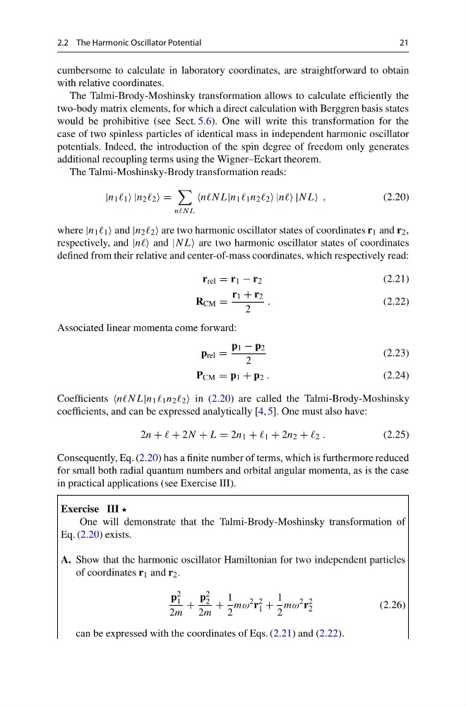
The Talmi-Moshinsky-Brody transformation reads:
|n 1 1 |n 2 2 =
nnNL
nnNL|n 1 1 n 2 2 |nn |NL ,
(2.20)
where |n 1 1 and |n 2 2 are two harmonic oscillator states of coordinates r 1 and r 2 ,
respectively, and |nn and |NL are two harmonic oscillator states of coordinates
defined from their relative and center-of-mass coordinates, which respectively read:
r rel = r 1 − r 2
(2.21)
R CM =
r 1 + r 2
2
.
(2.22)
Associated linear momenta come forward:
p rel =
p 1 − p 2
2
(2.23)
P CM = p 1 + p 2 .
(2.24)
Coefficients nnNL|n 1 1 n 2 2 in (2.20) are called the Talmi-Brody-Moshinsky
coefficients, and can be expressed analytically [4, 5]. One must also have:
2n + + 2N + L = 2n 1 + 1 + 2n 2 + 2 .
(2.25)
Consequently, Eq. (2.20) has a finite number of terms, which is furthermore reduced
for small both radial quantum numbers and orbital angular momenta, as is the case
in practical applications (see Exercise III).
Exercise III
One will demonstrate that the Talmi-Brody-Moshinsky transformation of
Eq. (2.20) exists.
A. Show that the harmonic oscillator Hamiltonian for two independent particles
of coordinates r 1 and r 2 .
p 2
1
2m
+
p 2
2
2m
+
1
2
mω
2 r
2
1 +
1
2
mω
2 r
2
2
(2.26)
can be expressed with the coordinates of Eqs. (2.21) and (2.22).
21
cumbersome to calculate in laboratory coordinates, are straightforward to obtain
with relative coordinates.
The Talmi-Brody-Moshinsky transformation allows to calculate efficiently the
two-body matrix elements, for which a direct calculation with Berggren basis states
would be prohibitive (see Sect. 5.6). One will write this transformation for the
case of two spinless particles of identical mass in independent harmonic oscillator
potentials. Indeed, the introduction of the spin degree of freedom only generates
additional recoupling terms using the Wigner–Eckart theorem.
The Talmi-Moshinsky-Brody transformation reads:
|n 1 1 |n 2 2 =
nnNL
nnNL|n 1 1 n 2 2 |nn |NL ,
(2.20)
where |n 1 1 and |n 2 2 are two harmonic oscillator states of coordinates r 1 and r 2 ,
respectively, and |nn and |NL are two harmonic oscillator states of coordinates
defined from their relative and center-of-mass coordinates, which respectively read:
r rel = r 1 − r 2
(2.21)
R CM =
r 1 + r 2
2
.
(2.22)
Associated linear momenta come forward:
p rel =
p 1 − p 2
2
(2.23)
P CM = p 1 + p 2 .
(2.24)
Coefficients nnNL|n 1 1 n 2 2 in (2.20) are called the Talmi-Brody-Moshinsky
coefficients, and can be expressed analytically [4, 5]. One must also have:
2n + + 2N + L = 2n 1 + 1 + 2n 2 + 2 .
(2.25)
Consequently, Eq. (2.20) has a finite number of terms, which is furthermore reduced
for small both radial quantum numbers and orbital angular momenta, as is the case
in practical applications (see Exercise III).
Exercise III
One will demonstrate that the Talmi-Brody-Moshinsky transformation of
Eq. (2.20) exists.
A. Show that the harmonic oscillator Hamiltonian for two independent particles
of coordinates r 1 and r 2 .
p 2
1
2m
+
p 2
2
2m
+
1
2
mω
2 r
2
1 +
1
2
mω
2 r
2
2
(2.26)
can be expressed with the coordinates of Eqs. (2.21) and (2.22).