

282
6 Physical Applications of the Gamow Shell Model
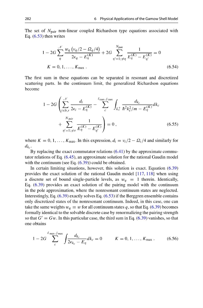
The set of N pair non-linear coupled Richardson type equations associated with
Eq. (6.53) then writes
1 − 2G
N
q
w q
ν q /2 − Ω q /4
2 q − E
(K)
η
+ 2G
N pair
η =1; =η
1
E
(K)
η
− E
(K)
η
= 0
K = 0, 1, . . . , K max .
(6.54)
The first sum in these equations can be separated in resonant and discretized
scattering parts. In the continuum limit, the generalized Richardson equations
become
1 − 2G
⎛
⎝
N
i∈b,r
d i
2 i − E
(K)
η
−
max ,j max
c
L
+
c
d k c
¯
h 2 k 2
c /m − E
(K)
η
dk c
+
N pair
η =1; =ν
1
E
(K)
η
− E
(K)
η
⎞
⎠ = 0 ,
(6.55)
where K = 0, 1, . . . , K max . In this expression, d i = ν i /2 − Ω i /4 and similarly for
d k c .
By replacing the exact commutator relations (6.41) by the approximate commutator relations of Eq. (6.45), an approximate solution for the rational Gaudin model
with the continuum (see Eq. (6.39)) could be obtained.
In certain limiting situations, however, this solution is exact. Equation (6.39)
provides the exact solution of the rational Gaudin model [117, 118] when using
a discrete set of bound single-particle levels, as w q = 1 therein. Identically,
Eq. (6.39) provides an exact solution of the pairing model with the continuum
in the pole approximation, where the nonresonant continuum states are neglected.
Interestingly, Eq. (6.39) exactly solves Eq. (6.53) if the Berggren ensemble contains
only discretized states of the nonresonant continuum. Indeed, in this case, one can
take the same weights w q ≡ w for all continuum states q, so that Eq. (6.39) becomes
formally identical to the solvable discrete case by renormalizing the pairing strength
so that G = Gw. In this particular case, the third sum in Eq. (6.39) vanishes, so that
one obtains
1 − 2G
max ,j max
c
d k c
2 k c − E η
dk c = 0
K = 0, 1, . . . , K max .
(6.56)
6 Physical Applications of the Gamow Shell Model
The set of N pair non-linear coupled Richardson type equations associated with
Eq. (6.53) then writes
1 − 2G
N
q
w q
ν q /2 − Ω q /4
2 q − E
(K)
η
+ 2G
N pair
η =1; =η
1
E
(K)
η
− E
(K)
η
= 0
K = 0, 1, . . . , K max .
(6.54)
The first sum in these equations can be separated in resonant and discretized
scattering parts. In the continuum limit, the generalized Richardson equations
become
1 − 2G
⎛
⎝
N
i∈b,r
d i
2 i − E
(K)
η
−
max ,j max
c
L
+
c
d k c
¯
h 2 k 2
c /m − E
(K)
η
dk c
+
N pair
η =1; =ν
1
E
(K)
η
− E
(K)
η
⎞
⎠ = 0 ,
(6.55)
where K = 0, 1, . . . , K max . In this expression, d i = ν i /2 − Ω i /4 and similarly for
d k c .
By replacing the exact commutator relations (6.41) by the approximate commutator relations of Eq. (6.45), an approximate solution for the rational Gaudin model
with the continuum (see Eq. (6.39)) could be obtained.
In certain limiting situations, however, this solution is exact. Equation (6.39)
provides the exact solution of the rational Gaudin model [117, 118] when using
a discrete set of bound single-particle levels, as w q = 1 therein. Identically,
Eq. (6.39) provides an exact solution of the pairing model with the continuum
in the pole approximation, where the nonresonant continuum states are neglected.
Interestingly, Eq. (6.39) exactly solves Eq. (6.53) if the Berggren ensemble contains
only discretized states of the nonresonant continuum. Indeed, in this case, one can
take the same weights w q ≡ w for all continuum states q, so that Eq. (6.39) becomes
formally identical to the solvable discrete case by renormalizing the pairing strength
so that G = Gw. In this particular case, the third sum in Eq. (6.39) vanishes, so that
one obtains
1 − 2G
max ,j max
c
d k c
2 k c − E η
dk c = 0
K = 0, 1, . . . , K max .
(6.56)