

236
5 Formulation and Implementation of the Gamow Shell Model
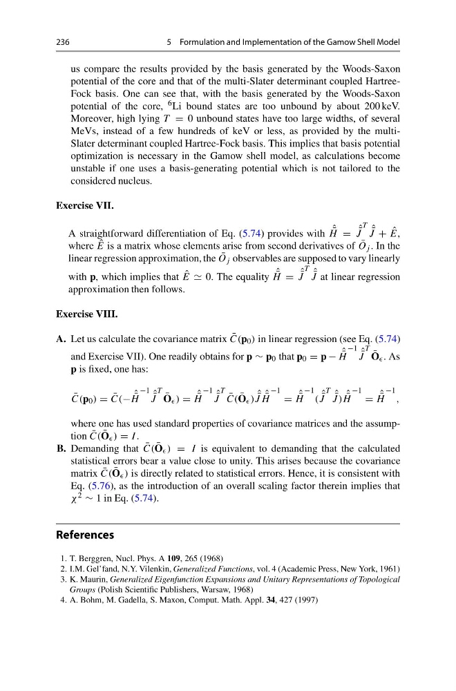
us compare the results provided by the basis generated by the Woods-Saxon
potential of the core and that of the multi-Slater determinant coupled HartreeFock basis. One can see that, with the basis generated by the Woods-Saxon
potential of the core, 6 Li bound states are too unbound by about 200 keV.
Moreover, high lying T = 0 unbound states have too large widths, of several
MeVs, instead of a few hundreds of keV or less, as provided by the multiSlater determinant coupled Hartree-Fock basis. This implies that basis potential
optimization is necessary in the Gamow shell model, as calculations become
unstable if one uses a basis-generating potential which is not tailored to the
considered nucleus.
Exercise VII.
A straightforward differentiation of Eq. (5.74) provides with ˆ ¯
H = ˆ ¯
J
T ˆ ¯
J + ˆ
E,
where ˆ
E is a matrix whose elements arise from second derivatives of ¯
O j . In the
linear regression approximation, the ¯
O j observables are supposed to vary linearly
with p, which implies that ˆ
E 0. The equality ˆ ¯
H = ˆ ¯
J
T ˆ ¯
J at linear regression
approximation then follows.
Exercise VIII.
A. Let us calculate the covariance matrix ¯
C(p 0 ) in linear regression (see Eq. (5.74)
and Exercise VII). One readily obtains for p ∼ p 0 that p 0 = p − ˆ ¯
H
−1
ˆ ¯
J
T ¯
O . As
p is fixed, one has:
¯
C(p 0 ) = ¯
C(− ˆ ¯
H
−1 ˆ ¯
J
T ¯
O ) = ˆ ¯
H
−1 ˆ ¯
J
T ¯
C( ¯
O ) ˆ ¯
J ˆ ¯
H
−1 = ˆ ¯
H
−1
( ˆ ¯
J
T ˆ ¯
J ) ˆ ¯
H
−1 = ˆ ¯
H
−1
,
where one has used standard properties of covariance matrices and the assumption ¯
C( ¯
O ) = I .
B. Demanding that ¯
C( ¯
O ) = I is equivalent to demanding that the calculated
statistical errors bear a value close to unity. This arises because the covariance
matrix ¯
C( ¯
O ) is directly related to statistical errors. Hence, it is consistent with
Eq. (5.76), as the introduction of an overall scaling factor therein implies that
χ 2 ∼ 1 in Eq. (5.74).
References
1. T. Berggren, Nucl. Phys. A 109, 265 (1968)
2. I.M. Gel’fand, N.Y. Vilenkin, Generalized Functions, vol. 4 (Academic Press, New York, 1961)
3. K. Maurin, Generalized Eigenfunction Expansions and Unitary Representations of Topological
Groups (Polish Scientific Publishers, Warsaw, 1968)
4. A. Bohm, M. Gadella, S. Maxon, Comput. Math. Appl. 34, 427 (1997)
5 Formulation and Implementation of the Gamow Shell Model
us compare the results provided by the basis generated by the Woods-Saxon
potential of the core and that of the multi-Slater determinant coupled HartreeFock basis. One can see that, with the basis generated by the Woods-Saxon
potential of the core, 6 Li bound states are too unbound by about 200 keV.
Moreover, high lying T = 0 unbound states have too large widths, of several
MeVs, instead of a few hundreds of keV or less, as provided by the multiSlater determinant coupled Hartree-Fock basis. This implies that basis potential
optimization is necessary in the Gamow shell model, as calculations become
unstable if one uses a basis-generating potential which is not tailored to the
considered nucleus.
Exercise VII.
A straightforward differentiation of Eq. (5.74) provides with ˆ ¯
H = ˆ ¯
J
T ˆ ¯
J + ˆ
E,
where ˆ
E is a matrix whose elements arise from second derivatives of ¯
O j . In the
linear regression approximation, the ¯
O j observables are supposed to vary linearly
with p, which implies that ˆ
E 0. The equality ˆ ¯
H = ˆ ¯
J
T ˆ ¯
J at linear regression
approximation then follows.
Exercise VIII.
A. Let us calculate the covariance matrix ¯
C(p 0 ) in linear regression (see Eq. (5.74)
and Exercise VII). One readily obtains for p ∼ p 0 that p 0 = p − ˆ ¯
H
−1
ˆ ¯
J
T ¯
O . As
p is fixed, one has:
¯
C(p 0 ) = ¯
C(− ˆ ¯
H
−1 ˆ ¯
J
T ¯
O ) = ˆ ¯
H
−1 ˆ ¯
J
T ¯
C( ¯
O ) ˆ ¯
J ˆ ¯
H
−1 = ˆ ¯
H
−1
( ˆ ¯
J
T ˆ ¯
J ) ˆ ¯
H
−1 = ˆ ¯
H
−1
,
where one has used standard properties of covariance matrices and the assumption ¯
C( ¯
O ) = I .
B. Demanding that ¯
C( ¯
O ) = I is equivalent to demanding that the calculated
statistical errors bear a value close to unity. This arises because the covariance
matrix ¯
C( ¯
O ) is directly related to statistical errors. Hence, it is consistent with
Eq. (5.76), as the introduction of an overall scaling factor therein implies that
χ 2 ∼ 1 in Eq. (5.74).
References
1. T. Berggren, Nucl. Phys. A 109, 265 (1968)
2. I.M. Gel’fand, N.Y. Vilenkin, Generalized Functions, vol. 4 (Academic Press, New York, 1961)
3. K. Maurin, Generalized Eigenfunction Expansions and Unitary Representations of Topological
Groups (Polish Scientific Publishers, Warsaw, 1968)
4. A. Bohm, M. Gadella, S. Maxon, Comput. Math. Appl. 34, 427 (1997)