

5.9 Diagonalization of Very Large Gamow Shell Model Matrices with the. . .
225
model space, one can reasonably assume that the density matrix renormalization
group used within the Gamow shell model will converge quickly. In fact, the
application of the density matrix renormalization group method in the Gamow shell
model is similar to that occurring in weakly coupled spin chains [40,41], in constrast
to the situation encountered in standard shell model, where couplings are large and
convergence slow [43–45].
The aim of the density matrix renormalization group method is to iteratively
build bases becoming more and more correlated. In these correlated bases, Gamow
shell model eigenstates can be expanded using a much smaller number of basis
states, typically a few thousands. For this, the Gamow shell model valence space
is separated in two spaces A and B. The space A is firstly constructed from the
one-body resonant states of the Berggren basis. One also has to add to the space
A a few one-body nonresonant states of quantum numbers , j different from
those of resonant states. These additional nonresonant states are necessary in order
to generate all possible couplings present in the Hamiltonian [39]. The space B
is generated during the density matrix renormalization group process, by adding
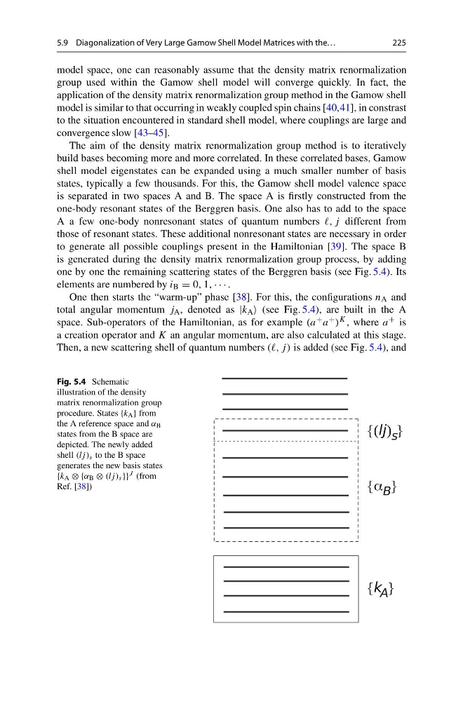
one by one the remaining scattering states of the Berggren basis (see Fig. 5.4). Its
elements are numbered by i B = 0, 1, · · · .
One then starts the “warm-up” phase [38]. For this, the configurations n A and
total angular momentum j A , denoted as |k A (see Fig. 5.4), are built in the A
space. Sub-operators of the Hamiltonian, as for example (a + a + ) K , where a + is
a creation operator and K an angular momentum, are also calculated at this stage.
Then, a new scattering shell of quantum numbers ((, j ) is added (see Fig. 5.4), and
Fig. 5.4 Schematic
illustration of the density
matrix renormalization group
procedure. States {k A } from
the A reference space and α B
states from the B space are
depicted. The newly added
shell (lj ) s to the B space
generates the new basis states
{k A ⊗ {α B ⊗ (lj ) s }} J (from
Ref. [38])
{ }
{ }
{
}
225
model space, one can reasonably assume that the density matrix renormalization
group used within the Gamow shell model will converge quickly. In fact, the
application of the density matrix renormalization group method in the Gamow shell
model is similar to that occurring in weakly coupled spin chains [40,41], in constrast
to the situation encountered in standard shell model, where couplings are large and
convergence slow [43–45].
The aim of the density matrix renormalization group method is to iteratively
build bases becoming more and more correlated. In these correlated bases, Gamow
shell model eigenstates can be expanded using a much smaller number of basis
states, typically a few thousands. For this, the Gamow shell model valence space
is separated in two spaces A and B. The space A is firstly constructed from the
one-body resonant states of the Berggren basis. One also has to add to the space
A a few one-body nonresonant states of quantum numbers , j different from
those of resonant states. These additional nonresonant states are necessary in order
to generate all possible couplings present in the Hamiltonian [39]. The space B
is generated during the density matrix renormalization group process, by adding
one by one the remaining scattering states of the Berggren basis (see Fig. 5.4). Its
elements are numbered by i B = 0, 1, · · · .
One then starts the “warm-up” phase [38]. For this, the configurations n A and
total angular momentum j A , denoted as |k A (see Fig. 5.4), are built in the A
space. Sub-operators of the Hamiltonian, as for example (a + a + ) K , where a + is
a creation operator and K an angular momentum, are also calculated at this stage.
Then, a new scattering shell of quantum numbers ((, j ) is added (see Fig. 5.4), and
Fig. 5.4 Schematic
illustration of the density
matrix renormalization group
procedure. States {k A } from
the A reference space and α B
states from the B space are
depicted. The newly added
shell (lj ) s to the B space
generates the new basis states
{k A ⊗ {α B ⊗ (lj ) s }} J (from
Ref. [38])
{ }
{ }
{
}