

70
4 Bateman Waves
curves are sometimes referred to as the t-lines on Minkowskian space-time. We
begin by defining the 4-vectors
E i = F ij u
j
= F i0 and B i =
∗ F ij u
j
=
∗ F i0 ,
(4.1)
where the dual of the tensor F ij , denoted ∗ F ij , is defined by
∗ F ij =
1
2
ij kl F
kl ,
(4.2)
and ij kl is the Levi–Civita permutation symbol in four dimensions with 0123 =
−1. Hence we have
E i = (0, E α ) = (0, F α0 ) ⇒ E
α
= F 0α ,
(4.3)
and
B i = (0, B α ) = (0,
∗ F α0 ) ⇒ B
α
=
∗ F 0α .
(4.4)
We shall henceforth take
E = (E
α ) = (E
1 , E
2 , E
3 ) and B = (B
α ) = (B
1 , B
2 , B
3 ) .
(4.5)
We note that with our convention for raising and lowering indices E α = −E α ,
B α = −B α and we have also used the skew symmetry of F ij and ∗ F ij . From (4.3)
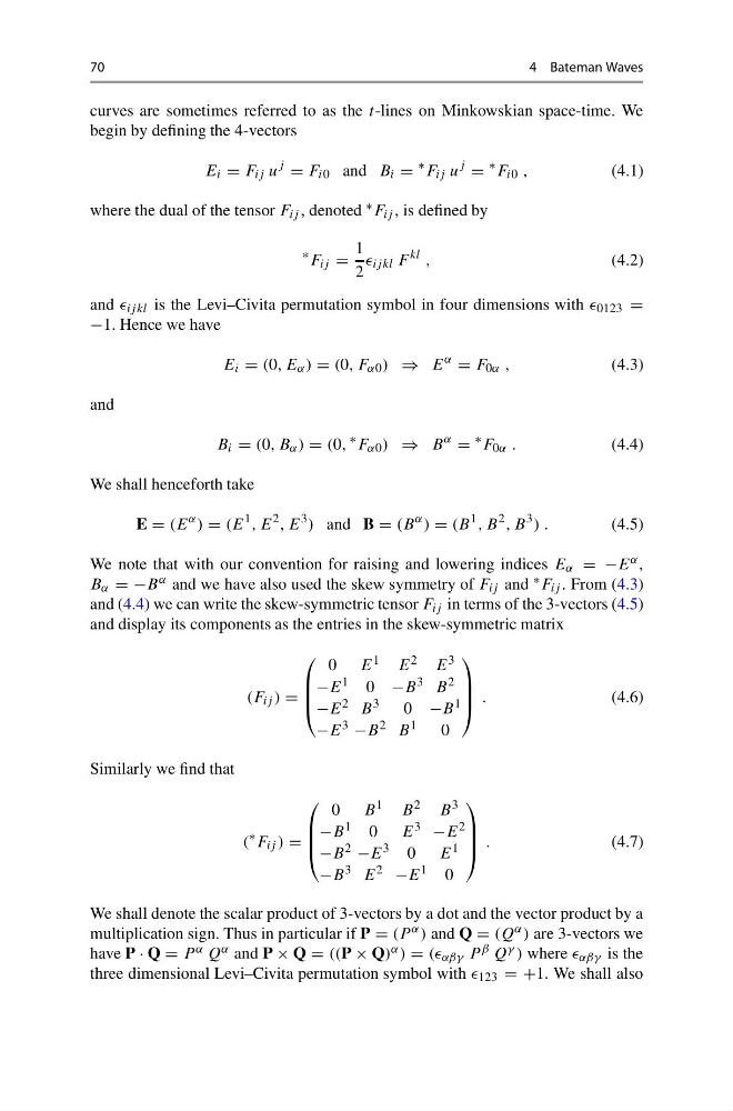
and (4.4) we can write the skew-symmetric tensor F ij in terms of the 3-vectors (4.5)
and display its components as the entries in the skew-symmetric matrix
(F ij ) =
⎛
⎜
⎜
⎝
0 E 1 E 2 E 3
−E 1 0 −B 3 B 2
−E 2 B 3 0 −B 1
−E 3 −B 2 B 1 0
⎞
⎟
⎟
⎠ .
(4.6)
Similarly we find that
(
∗ F ij ) =
⎛
⎜
⎜
⎝
0 B 1 B 2 B 3
−B 1 0 E 3 −E 2
−B 2 −E 3 0 E 1
−B 3 E 2 −E 1 0
⎞
⎟
⎟
⎠ .
(4.7)
We shall denote the scalar product of 3-vectors by a dot and the vector product by a
multiplication sign. Thus in particular if P = (P α ) and Q = (Q α ) are 3-vectors we
have P · Q = P α Q α and P × Q = ((P × Q) α ) = (( αβγ P β Q γ ) where αβγ is the
three dimensional Levi–Civita permutation symbol with 123 = +1. We shall also
4 Bateman Waves
curves are sometimes referred to as the t-lines on Minkowskian space-time. We
begin by defining the 4-vectors
E i = F ij u
j
= F i0 and B i =
∗ F ij u
j
=
∗ F i0 ,
(4.1)
where the dual of the tensor F ij , denoted ∗ F ij , is defined by
∗ F ij =
1
2
ij kl F
kl ,
(4.2)
and ij kl is the Levi–Civita permutation symbol in four dimensions with 0123 =
−1. Hence we have
E i = (0, E α ) = (0, F α0 ) ⇒ E
α
= F 0α ,
(4.3)
and
B i = (0, B α ) = (0,
∗ F α0 ) ⇒ B
α
=
∗ F 0α .
(4.4)
We shall henceforth take
E = (E
α ) = (E
1 , E
2 , E
3 ) and B = (B
α ) = (B
1 , B
2 , B
3 ) .
(4.5)
We note that with our convention for raising and lowering indices E α = −E α ,
B α = −B α and we have also used the skew symmetry of F ij and ∗ F ij . From (4.3)
and (4.4) we can write the skew-symmetric tensor F ij in terms of the 3-vectors (4.5)
and display its components as the entries in the skew-symmetric matrix
(F ij ) =
⎛
⎜
⎜
⎝
0 E 1 E 2 E 3
−E 1 0 −B 3 B 2
−E 2 B 3 0 −B 1
−E 3 −B 2 B 1 0
⎞
⎟
⎟
⎠ .
(4.6)
Similarly we find that
(
∗ F ij ) =
⎛
⎜
⎜
⎝
0 B 1 B 2 B 3
−B 1 0 E 3 −E 2
−B 2 −E 3 0 E 1
−B 3 E 2 −E 1 0
⎞
⎟
⎟
⎠ .
(4.7)
We shall denote the scalar product of 3-vectors by a dot and the vector product by a
multiplication sign. Thus in particular if P = (P α ) and Q = (Q α ) are 3-vectors we
have P · Q = P α Q α and P × Q = ((P × Q) α ) = (( αβγ P β Q γ ) where αβγ is the
three dimensional Levi–Civita permutation symbol with 123 = +1. We shall also