

14
1 Congruences of World Lines
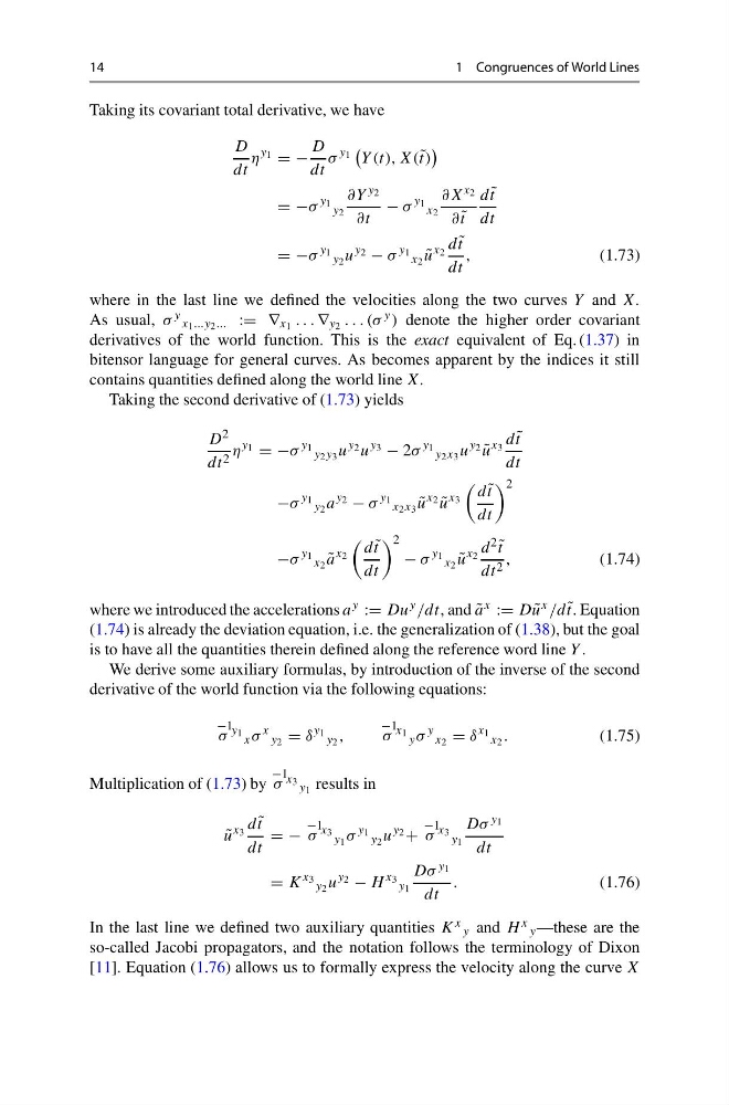
Taking its covariant total derivative, we have
D
dt
η
y 1 = −
D
dt
σ
y 1
Y (t), X(˜ t)
= −σ
y 1 y 2
∂Y y 2
∂t
− σ
y 1 x 2
∂X x 2
∂ ˜
t
d ˜
t
dt
= −σ
y 1 y 2 u
y 2 − σ
y 1 x 2 ˜
u
x 2
d ˜
t
dt
,
(1.73)
where in the last line we defined the velocities along the two curves Y and X.
As usual, σ y x 1 ...y 2 ... := ∇ x 1 . . . ∇ y 2 . . . (σ y ) denote the higher order covariant
derivatives of the world function. This is the exact equivalent of Eq. (1.37) in
bitensor language for general curves. As becomes apparent by the indices it still
contains quantities defined along the world line X.
Taking the second derivative of (1.73) yields
D 2
dt 2 η
y 1 = −σ
y 1 y 2 y 3 u
y 2 u
y 3 − 2σ
y 1 y 2 x 3 u
y 2 ˜
u
x 3
d ˜
t
dt
−σ
y 1 y 2 a
y 2 − σ
y 1 x 2 x 3 ˜
u
x 2 ˜
u
x 3
d ˜
t
dt
2
−σ
y 1 x 2 ˜
a
x 2
d ˜
t
dt
2
− σ
y 1 x 2 ˜
u
x 2
d 2 ˜
t
dt 2 ,
(1.74)
where we introduced the accelerations a y := Du y /dt, and ˜
a x := D ˜
u x /d ˜
t. Equation
(1.74) is already the deviation equation, i.e. the generalization of (1.38), but the goal
is to have all the quantities therein defined along the reference word line Y .
We derive some auxiliary formulas, by introduction of the inverse of the second
derivative of the world function via the following equations:
−1
σ
y 1 x σ
x
y 2 = δ
y 1 y 2 ,
−1
σ
x 1 y σ
y
x 2 = δ
x 1 x 2 .
(1.75)
Multiplication of (1.73) by
−1
σ x 3 y 1 results in
˜
u
x 3
d ˜
t
dt
= −
−1
σ
x 3 y 1 σ
y 1 y 2 u
y 2 +
−1
σ
x 3 y 1
Dσ y 1
dt
= K
x 3 y 2 u
y 2 − H
x 3 y 1
Dσ y 1
dt
.
(1.76)
In the last line we defined two auxiliary quantities K x y and H x y —these are the
so-called Jacobi propagators, and the notation follows the terminology of Dixon
[11]. Equation (1.76) allows us to formally express the velocity along the curve X
1 Congruences of World Lines
Taking its covariant total derivative, we have
D
dt
η
y 1 = −
D
dt
σ
y 1
Y (t), X(˜ t)
= −σ
y 1 y 2
∂Y y 2
∂t
− σ
y 1 x 2
∂X x 2
∂ ˜
t
d ˜
t
dt
= −σ
y 1 y 2 u
y 2 − σ
y 1 x 2 ˜
u
x 2
d ˜
t
dt
,
(1.73)
where in the last line we defined the velocities along the two curves Y and X.
As usual, σ y x 1 ...y 2 ... := ∇ x 1 . . . ∇ y 2 . . . (σ y ) denote the higher order covariant
derivatives of the world function. This is the exact equivalent of Eq. (1.37) in
bitensor language for general curves. As becomes apparent by the indices it still
contains quantities defined along the world line X.
Taking the second derivative of (1.73) yields
D 2
dt 2 η
y 1 = −σ
y 1 y 2 y 3 u
y 2 u
y 3 − 2σ
y 1 y 2 x 3 u
y 2 ˜
u
x 3
d ˜
t
dt
−σ
y 1 y 2 a
y 2 − σ
y 1 x 2 x 3 ˜
u
x 2 ˜
u
x 3
d ˜
t
dt
2
−σ
y 1 x 2 ˜
a
x 2
d ˜
t
dt
2
− σ
y 1 x 2 ˜
u
x 2
d 2 ˜
t
dt 2 ,
(1.74)
where we introduced the accelerations a y := Du y /dt, and ˜
a x := D ˜
u x /d ˜
t. Equation
(1.74) is already the deviation equation, i.e. the generalization of (1.38), but the goal
is to have all the quantities therein defined along the reference word line Y .
We derive some auxiliary formulas, by introduction of the inverse of the second
derivative of the world function via the following equations:
−1
σ
y 1 x σ
x
y 2 = δ
y 1 y 2 ,
−1
σ
x 1 y σ
y
x 2 = δ
x 1 x 2 .
(1.75)
Multiplication of (1.73) by
−1
σ x 3 y 1 results in
˜
u
x 3
d ˜
t
dt
= −
−1
σ
x 3 y 1 σ
y 1 y 2 u
y 2 +
−1
σ
x 3 y 1
Dσ y 1
dt
= K
x 3 y 2 u
y 2 − H
x 3 y 1
Dσ y 1
dt
.
(1.76)
In the last line we defined two auxiliary quantities K x y and H x y —these are the
so-called Jacobi propagators, and the notation follows the terminology of Dixon
[11]. Equation (1.76) allows us to formally express the velocity along the curve X