

230
C Gravitational (Clock) Compass
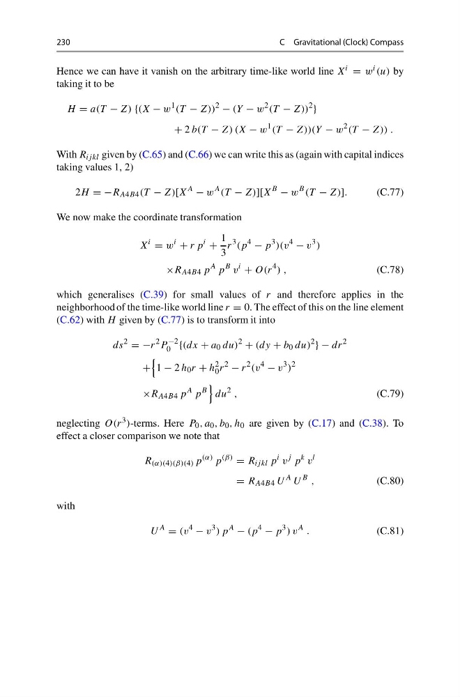
Hence we can have it vanish on the arbitrary time-like world line X i = w i (u) by
taking it to be
H = a(T − Z) {(X − w
1 (T − Z))
2
− (Y − w
2 (T − Z))
2
}
+ 2 b(T − Z) (X − w
1 (T − Z))(Y − w
2 (T − Z)) .
With R ij kl given by (C.65) and (C.66) we can write this as (again with capital indices
taking values 1, 2)
2H = −R A4B4 (T − Z)[X
A
− w
A (T − Z)][X
B
− w
B (T − Z)].
(C.77)
We now make the coordinate transformation
X
i
= w
i
+ r p
i
+
1
3
r
3 (p
4
− p
3 )(v
4
− v
3 )
×R A4B4 p
A p
B v
i
+ O(r
4 ) ,
(C.78)
which generalises (C.39) for small values of r and therefore applies in the
neighborhood of the time-like world line r = 0. The effect of this on the line element
(C.62) with H given by (C.77) is to transform it into
ds
2
= −r
2 P
−2
0 {(dx + a 0 du)
2
+ (dy + b 0 du)
2
} − dr
2
+
1 − 2 h 0 r + h
2
0 r
2
− r
2 (v
4
− v
3 )
2
×R A4B4 p
A p
B
du
2 ,
(C.79)
neglecting O(r 3 )-terms. Here P 0 , a 0 , b 0 , h 0 are given by (C.17) and (C.38). To
effect a closer comparison we note that
R (α)(4)(β)(4) p
(α) p
(β)
= R ij kl p
i v
j p
k v
l
= R A4B4 U
A U
B ,
(C.80)
with
U
A
= (v
4
− v
3 ) p
A
− (p
4
− p
3 ) v
A .
(C.81)
C Gravitational (Clock) Compass
Hence we can have it vanish on the arbitrary time-like world line X i = w i (u) by
taking it to be
H = a(T − Z) {(X − w
1 (T − Z))
2
− (Y − w
2 (T − Z))
2
}
+ 2 b(T − Z) (X − w
1 (T − Z))(Y − w
2 (T − Z)) .
With R ij kl given by (C.65) and (C.66) we can write this as (again with capital indices
taking values 1, 2)
2H = −R A4B4 (T − Z)[X
A
− w
A (T − Z)][X
B
− w
B (T − Z)].
(C.77)
We now make the coordinate transformation
X
i
= w
i
+ r p
i
+
1
3
r
3 (p
4
− p
3 )(v
4
− v
3 )
×R A4B4 p
A p
B v
i
+ O(r
4 ) ,
(C.78)
which generalises (C.39) for small values of r and therefore applies in the
neighborhood of the time-like world line r = 0. The effect of this on the line element
(C.62) with H given by (C.77) is to transform it into
ds
2
= −r
2 P
−2
0 {(dx + a 0 du)
2
+ (dy + b 0 du)
2
} − dr
2
+
1 − 2 h 0 r + h
2
0 r
2
− r
2 (v
4
− v
3 )
2
×R A4B4 p
A p
B
du
2 ,
(C.79)
neglecting O(r 3 )-terms. Here P 0 , a 0 , b 0 , h 0 are given by (C.17) and (C.38). To
effect a closer comparison we note that
R (α)(4)(β)(4) p
(α) p
(β)
= R ij kl p
i v
j p
k v
l
= R A4B4 U
A U
B ,
(C.80)
with
U
A
= (v
4
− v
3 ) p
A
− (p
4
− p
3 ) v
A .
(C.81)