

7.4 Equations of Motion in First Approximation
167
E (2)(3) =
g
r 2 P 0
∗ F ij (u) k
i ∂k j
∂y
+ O
1
r
,
(7.113)
E (3)(3) = O(r
0 ) ,
(7.114)
E (1)(4) = −
g
r 2 P 0
∗ F ij (u) (v
i
−
1
2
k
i )
∂k j
∂x
+ O
1
r
,
(7.115)
E (2)(4) = −
g
r 2 P 0
∗ F ij (u) (v
i
−
1
2
k
i )
∂k j
∂y
+ O
1
r
,
(7.116)
E (3)(4) =
g
r 2
∗ F ij (u) k
i v
j
+ O
1
r
, E 44 = O
1
r
.
(7.117)
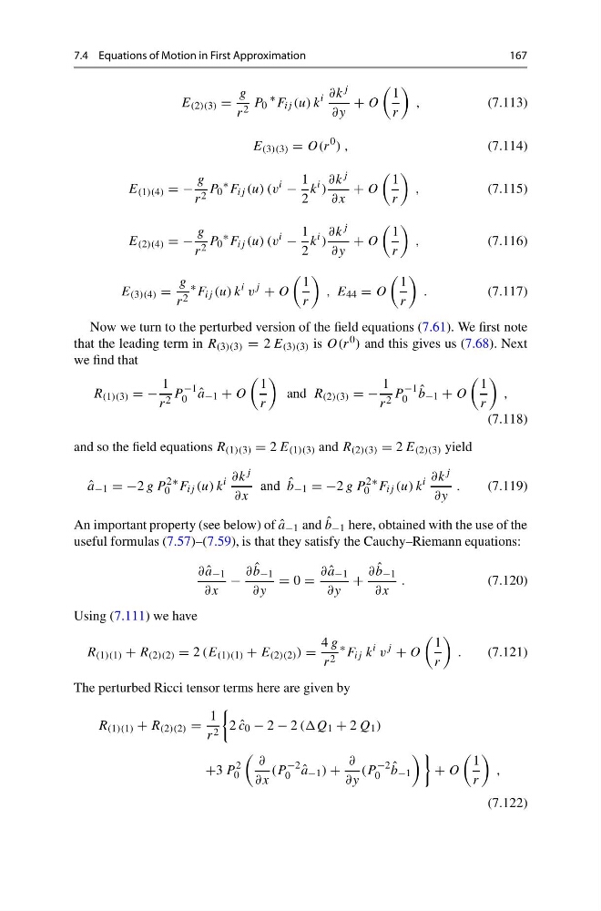
Now we turn to the perturbed version of the field equations (7.61). We first note
that the leading term in R (3)(3) = 2 E (3)(3) is O(r 0 ) and this gives us (7.68). Next
we find that
R (1)(3) = −
1
r 2 P
−1
0 ˆ
a −1 + O
1
r
and R (2)(3) = −
1
r 2 P
−1
0
ˆ
b −1 + O
1
r
,
(7.118)
and so the field equations R (1)(3) = 2 E (1)(3) and R (2)(3) = 2 E (2)(3) yield
ˆ
a −1 = −2 g P
2
0
∗ F ij (u) k
i ∂k j
∂x
and ˆ
b −1 = −2 g P
2
0
∗ F ij (u) k
i ∂k j
∂y
.
(7.119)
An important property (see below) of ˆ
a −1 and ˆ
b −1 here, obtained with the use of the
useful formulas (7.57)–(7.59), is that they satisfy the Cauchy–Riemann equations:
∂ ˆ
a −1
∂x
−
∂ ˆ
b −1
∂y
= 0 =
∂ ˆ
a −1
∂y
+
∂ ˆ
b −1
∂x
.
(7.120)
Using (7.111) we have
R (1)(1) + R (2)(2) = 2 (E (1)(1) + E (2)(2) ) =
4 g
r 2
∗ F ij k
i v
j
+ O
1
r
.
(7.121)
The perturbed Ricci tensor terms here are given by
R (1)(1) + R (2)(2) =
1
r 2
2 ˆ
c 0 − 2 − 2 ((Q 1 + 2 Q 1 )
+3 P
2
0
∂
∂x
(P
−2
0 ˆ
a −1 ) +
∂
∂y
(P
−2
0
ˆ
b −1
+ O
1
r
,
(7.122)
167
E (2)(3) =
g
r 2 P 0
∗ F ij (u) k
i ∂k j
∂y
+ O
1
r
,
(7.113)
E (3)(3) = O(r
0 ) ,
(7.114)
E (1)(4) = −
g
r 2 P 0
∗ F ij (u) (v
i
−
1
2
k
i )
∂k j
∂x
+ O
1
r
,
(7.115)
E (2)(4) = −
g
r 2 P 0
∗ F ij (u) (v
i
−
1
2
k
i )
∂k j
∂y
+ O
1
r
,
(7.116)
E (3)(4) =
g
r 2
∗ F ij (u) k
i v
j
+ O
1
r
, E 44 = O
1
r
.
(7.117)
Now we turn to the perturbed version of the field equations (7.61). We first note
that the leading term in R (3)(3) = 2 E (3)(3) is O(r 0 ) and this gives us (7.68). Next
we find that
R (1)(3) = −
1
r 2 P
−1
0 ˆ
a −1 + O
1
r
and R (2)(3) = −
1
r 2 P
−1
0
ˆ
b −1 + O
1
r
,
(7.118)
and so the field equations R (1)(3) = 2 E (1)(3) and R (2)(3) = 2 E (2)(3) yield
ˆ
a −1 = −2 g P
2
0
∗ F ij (u) k
i ∂k j
∂x
and ˆ
b −1 = −2 g P
2
0
∗ F ij (u) k
i ∂k j
∂y
.
(7.119)
An important property (see below) of ˆ
a −1 and ˆ
b −1 here, obtained with the use of the
useful formulas (7.57)–(7.59), is that they satisfy the Cauchy–Riemann equations:
∂ ˆ
a −1
∂x
−
∂ ˆ
b −1
∂y
= 0 =
∂ ˆ
a −1
∂y
+
∂ ˆ
b −1
∂x
.
(7.120)
Using (7.111) we have
R (1)(1) + R (2)(2) = 2 (E (1)(1) + E (2)(2) ) =
4 g
r 2
∗ F ij k
i v
j
+ O
1
r
.
(7.121)
The perturbed Ricci tensor terms here are given by
R (1)(1) + R (2)(2) =
1
r 2
2 ˆ
c 0 − 2 − 2 ((Q 1 + 2 Q 1 )
+3 P
2
0
∂
∂x
(P
−2
0 ˆ
a −1 ) +
∂
∂y
(P
−2
0
ˆ
b −1
+ O
1
r
,
(7.122)