

5.4 Gravitational Clock Compass
113
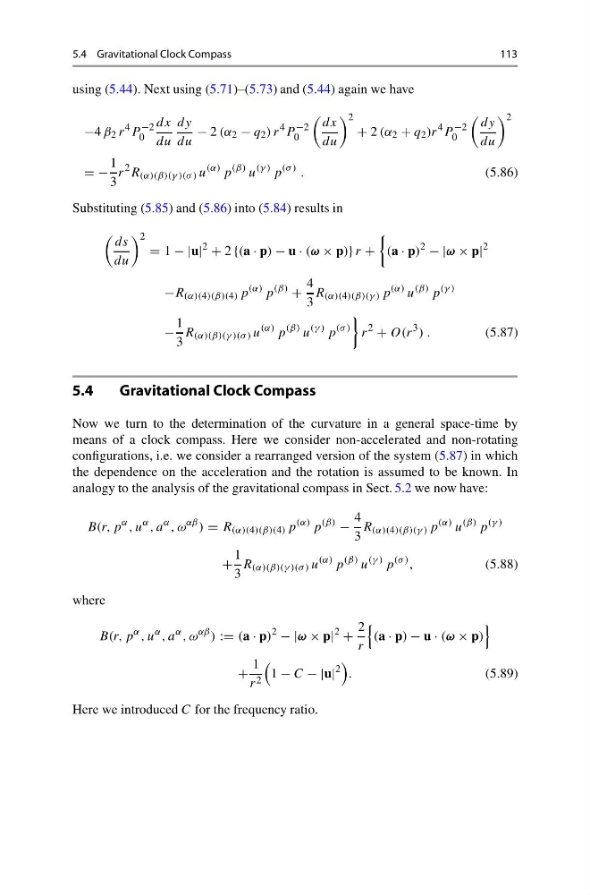
using (5.44). Next using (5.71)–(5.73) and (5.44) again we have
−4 β 2 r
4 P
−2
0
dx
du
dy
du
− 2 (α 2 − q 2 ) r
4 P
−2
0
dx
du
2
+ 2 (α 2 + q 2 )r
4 P
−2
0
dy
du
2
= −
1
3
r
2 R (α)(β)(γ )(σ ) u
(α) p
(β) u
(γ ) p
(σ ) .
(5.86)
Substituting (5.85) and (5.86) into (5.84) results in
ds
du
2
= 1 − |u|
2
+ 2 {(a · p) − u · (ω × p)} r +
(a · p)
2
− |ω × p|
2
−R (α)(4)(β)(4) p
(α) p
(β)
+
4
3
R (α)(4)(β)(γ ) p
(α) u
(β) p
(γ )
−
1
3
R (α)(β)(γ )(σ ) u
(α) p
(β) u
(γ ) p
(σ )
r
2
+ O(r
3 ) .
(5.87)
5.4
Gravitational Clock Compass
Now we turn to the determination of the curvature in a general space-time by
means of a clock compass. Here we consider non-accelerated and non-rotating
configurations, i.e. we consider a rearranged version of the system (5.87) in which
the dependence on the acceleration and the rotation is assumed to be known. In
analogy to the analysis of the gravitational compass in Sect. 5.2 we now have:
B(r, p
α , u
α , a
α , ω
αβ ) = R (α)(4)(β)(4) p
(α) p
(β)
−
4
3
R (α)(4)(β)(γ ) p
(α) u
(β) p
(γ )
+
1
3
R (α)(β)(γ )(σ ) u
(α) p
(β) u
(γ ) p
(σ ) ,
(5.88)
where
B(r, p
α , u
α , a
α , ω
αβ ) := (a · p)
2
− |ω × p|
2
+
2
r
(a · p) − u · (ω × p)
+
1
r 2
1 − C − |u|
2
.
(5.89)
Here we introduced C for the frequency ratio.
113
using (5.44). Next using (5.71)–(5.73) and (5.44) again we have
−4 β 2 r
4 P
−2
0
dx
du
dy
du
− 2 (α 2 − q 2 ) r
4 P
−2
0
dx
du
2
+ 2 (α 2 + q 2 )r
4 P
−2
0
dy
du
2
= −
1
3
r
2 R (α)(β)(γ )(σ ) u
(α) p
(β) u
(γ ) p
(σ ) .
(5.86)
Substituting (5.85) and (5.86) into (5.84) results in
ds
du
2
= 1 − |u|
2
+ 2 {(a · p) − u · (ω × p)} r +
(a · p)
2
− |ω × p|
2
−R (α)(4)(β)(4) p
(α) p
(β)
+
4
3
R (α)(4)(β)(γ ) p
(α) u
(β) p
(γ )
−
1
3
R (α)(β)(γ )(σ ) u
(α) p
(β) u
(γ ) p
(σ )
r
2
+ O(r
3 ) .
(5.87)
5.4
Gravitational Clock Compass
Now we turn to the determination of the curvature in a general space-time by
means of a clock compass. Here we consider non-accelerated and non-rotating
configurations, i.e. we consider a rearranged version of the system (5.87) in which
the dependence on the acceleration and the rotation is assumed to be known. In
analogy to the analysis of the gravitational compass in Sect. 5.2 we now have:
B(r, p
α , u
α , a
α , ω
αβ ) = R (α)(4)(β)(4) p
(α) p
(β)
−
4
3
R (α)(4)(β)(γ ) p
(α) u
(β) p
(γ )
+
1
3
R (α)(β)(γ )(σ ) u
(α) p
(β) u
(γ ) p
(σ ) ,
(5.88)
where
B(r, p
α , u
α , a
α , ω
αβ ) := (a · p)
2
− |ω × p|
2
+
2
r
(a · p) − u · (ω × p)
+
1
r 2
1 − C − |u|
2
.
(5.89)
Here we introduced C for the frequency ratio.