

362
C.-F. Dobrescu
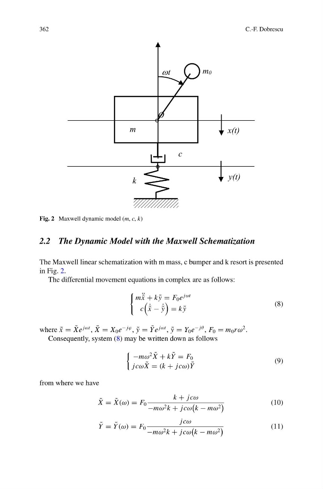
Fig. 2 Maxwell dynamic model (m, c, k)
2.2 The Dynamic Model with the Maxwell Schematization
The Maxwell linear schematization with m mass, c bumper and k resort is presented
in Fig. 2.
The differential movement equations in complex are as follows:
m ¨ ˜
x + k ˜
y = F 0 e
jωt
c
˙ ˜
x − ˙ ˜
y
= k ˜
y
(8)
where ˜
x = ˜
Xe
jωt , ˜
X = X 0 e
− jϕ , ˜
y = ˜
Y e
jωt , ˜
y = Y 0 e
− jθ , F 0 = m 0 r ω
2 .
Consequently, system (8) may be written down as follows
−mω
2 ˜
X + k ˜
Y = F 0
jcω ˜
X = (k + jcω) ˜
Y
(9)
from where we have
˜
X = ˜
X (ω) = F 0
k + jcω
−mω 2 k + jcω
k − mω 2
(10)
˜
Y = ˜
Y (ω) = F 0
jcω
−mω 2 k + jcω
k − mω 2
(11)
C.-F. Dobrescu
Fig. 2 Maxwell dynamic model (m, c, k)
2.2 The Dynamic Model with the Maxwell Schematization
The Maxwell linear schematization with m mass, c bumper and k resort is presented
in Fig. 2.
The differential movement equations in complex are as follows:
m ¨ ˜
x + k ˜
y = F 0 e
jωt
c
˙ ˜
x − ˙ ˜
y
= k ˜
y
(8)
where ˜
x = ˜
Xe
jωt , ˜
X = X 0 e
− jϕ , ˜
y = ˜
Y e
jωt , ˜
y = Y 0 e
− jθ , F 0 = m 0 r ω
2 .
Consequently, system (8) may be written down as follows
−mω
2 ˜
X + k ˜
Y = F 0
jcω ˜
X = (k + jcω) ˜
Y
(9)
from where we have
˜
X = ˜
X (ω) = F 0
k + jcω
−mω 2 k + jcω
k − mω 2
(10)
˜
Y = ˜
Y (ω) = F 0
jcω
−mω 2 k + jcω
k − mω 2
(11)