

360
C.-F. Dobrescu
2 The Parametric Analysis of the Compaction Process
for the Vibratory-Field Roller System
Based on experimental and numerical, research, on the rheological modeling and
the dynamic capability of vibratory rollers, there can be used, in a first approach,
the viscoelastic linear models made of a viscoelastic resort-bumper system with the
series connection.
2.1 The Dynamic Model with Voigt–Kelvin Schematics
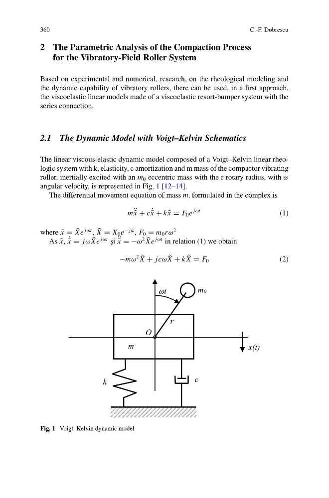
The linear viscous-elastic dynamic model composed of a Voigt–Kelvin linear rheologic system with k, elasticity, c amortization and m mass of the compactor vibrating
roller, inertially excited with an m 0 eccentric mass with the r rotary radius, with ω
angular velocity, is represented in Fig. 1 [12–14].
The differential movement equation of mass m, formulated in the complex is
m ¨ ˜
x + c ˙ ˜
x + k ˜
x = F 0 e
jωt
(1)
where ˜
x = ˜
Xe
jωt , ˜
X = X 0 e
− jϕ , F 0 = m 0 r ω
2
As ˜
x, ˙ ˜
x = jω ˜
Xe
jωt ¸
si ¨ ˜
x = −ω
2 ˜
Xe
jωt in relation (1) we obtain
−mω
2 ˜
X + jcω ˜
X + k ˜
X = F 0
(2)
Fig. 1 Voigt–Kelvin dynamic model
C.-F. Dobrescu
2 The Parametric Analysis of the Compaction Process
for the Vibratory-Field Roller System
Based on experimental and numerical, research, on the rheological modeling and
the dynamic capability of vibratory rollers, there can be used, in a first approach,
the viscoelastic linear models made of a viscoelastic resort-bumper system with the
series connection.
2.1 The Dynamic Model with Voigt–Kelvin Schematics
The linear viscous-elastic dynamic model composed of a Voigt–Kelvin linear rheologic system with k, elasticity, c amortization and m mass of the compactor vibrating
roller, inertially excited with an m 0 eccentric mass with the r rotary radius, with ω
angular velocity, is represented in Fig. 1 [12–14].
The differential movement equation of mass m, formulated in the complex is
m ¨ ˜
x + c ˙ ˜
x + k ˜
x = F 0 e
jωt
(1)
where ˜
x = ˜
Xe
jωt , ˜
X = X 0 e
− jϕ , F 0 = m 0 r ω
2
As ˜
x, ˙ ˜
x = jω ˜
Xe
jωt ¸
si ¨ ˜
x = −ω
2 ˜
Xe
jωt in relation (1) we obtain
−mω
2 ˜
X + jcω ˜
X + k ˜
X = F 0
(2)
Fig. 1 Voigt–Kelvin dynamic model