

108
E. Chircan et al.
([m 11 ] + [m 22 ])
¨
δ e
+ 2ω([m 21 ] − [m 12 ])
˙
δ e
+
[k e ] + ε([m 21 ] − [m 12 ]) − ω
2
([m 11 ] + (m 22 ))
= {q e } +
q
∗
e
−
q
i
e (ε)
−
q
i
e
ω
2
−
m
i
Ee
[I ]{ε} L
− [m oe ][R]
T
{¨ r o }
(31)
where:
m
i
oe
=
L
0
ρ A[N ]
T dx;
m
i
Ee
=
L
0
[N ]
∗ dx;
m i j
=
L
0
[N i ]
T
N j
ρ Adx
i, j = 1, 2, 3
q
∗
e
=
L
0
p x p y p z m x m y m z
N
N
∗
dx
(32)
3 Eigenvalues and Domain of Stability
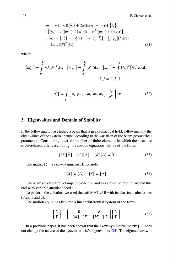
In the following, it was studied a beam that is in a centrifugal field, following how the
eigenvalues of the system change according to the variation of the beam geometrical
parameters. Considering a certain number of finite elements in which the structure
is discretized, after assembling, the motion equations will be of the form:
[M]
¨
+ [C]
˙
+ [K ]{} = 0
(33)
The matrix [C] is skew-symmetric. If we note:
{X } = {}; {Y } =
˙
(34)
The beam is considered clamped to one end and has a rotation motion around this
end with variable angular speed ω.
To perform the calculus, we used the soft MATLAB with its classical subroutines
(Figs. 1 and 2).
The motion equations become a linear differential system of the form:
˙
X
˙
Y
=
0
E
−[M]
−1 [K ] −[M]
−1 [C]
X
Y
(35)
In a previous paper, it has been shown that the skew-symmetric matrix [C] does
not change the nature of the system matrix’s eigenvalues (35). The eigenvalues will
E. Chircan et al.
([m 11 ] + [m 22 ])
¨
δ e
+ 2ω([m 21 ] − [m 12 ])
˙
δ e
+
[k e ] + ε([m 21 ] − [m 12 ]) − ω
2
([m 11 ] + (m 22 ))
= {q e } +
q
∗
e
−
q
i
e (ε)
−
q
i
e
ω
2
−
m
i
Ee
[I ]{ε} L
− [m oe ][R]
T
{¨ r o }
(31)
where:
m
i
oe
=
L
0
ρ A[N ]
T dx;
m
i
Ee
=
L
0
[N ]
∗ dx;
m i j
=
L
0
[N i ]
T
N j
ρ Adx
i, j = 1, 2, 3
q
∗
e
=
L
0
p x p y p z m x m y m z
N
N
∗
dx
(32)
3 Eigenvalues and Domain of Stability
In the following, it was studied a beam that is in a centrifugal field, following how the
eigenvalues of the system change according to the variation of the beam geometrical
parameters. Considering a certain number of finite elements in which the structure
is discretized, after assembling, the motion equations will be of the form:
[M]
¨
+ [C]
˙
+ [K ]{} = 0
(33)
The matrix [C] is skew-symmetric. If we note:
{X } = {}; {Y } =
˙
(34)
The beam is considered clamped to one end and has a rotation motion around this
end with variable angular speed ω.
To perform the calculus, we used the soft MATLAB with its classical subroutines
(Figs. 1 and 2).
The motion equations become a linear differential system of the form:
˙
X
˙
Y
=
0
E
−[M]
−1 [K ] −[M]
−1 [C]
X
Y
(35)
In a previous paper, it has been shown that the skew-symmetric matrix [C] does
not change the nature of the system matrix’s eigenvalues (35). The eigenvalues will