

Dynamical Response of a Beam in a Centrifugal Field …
103
where β 1 , γ 1 and β 2 , γ 2 are the slopes of the ends of the beam; α 1 and α 2 represent
the torsion of the end sections; m xOz1 , m xOy1 and m xOz2 , m xOy2 are the curvatures in
the corresponding plane.
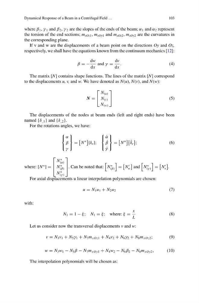
If v and w are the displacements of a beam point on the directions Oy and Oz,
respectively, we shall have the equations known from the continuum mechanics [12]:
β = −
dw
dx
and γ =
dv
dx
.
(4)
The matrix [N] contains shape functions. The lines of the matrix [N] correspond
to the displacements u, v, and w. We have denoted as N(u), N(v), and N(w):
N =
⎡
⎣
N (u)
N (v)
N (w)
⎤
⎦
(5)
The displacements of the nodes at beam ends (left and right ends) have been
named {δ _1 } and {δ _2 }.
For the rotations angles, we have:
⎧
⎨
⎩
α
β
γ
⎫
⎬
⎭
=
N
∗
{δ e };
⎧
⎨
⎩
˙
α
˙
β
˙
γ
⎫
⎬
⎭
=
N
∗
˙
δ e
;
(6)
where: [N
∗ ] =
⎡
⎢
⎣
N
∗
(α)
N
∗
(β)
N
∗
(γ )
⎤
⎥
⎦. Can be noted that:
N
∗
(β)
=
N
w
and
N
∗
(γ )
=
N
v
.
For axial displacements u linear interpolation polynomials are chosen:
u = N 1 u 1 + N 2 u 2
(7)
with:
N 1 = 1 − ξ ; N 1 = ξ ; where: ξ =
x
L
(8)
Let us consider now the transversal displacements v and w:
v = N 3 v 1 + N 5 γ 1 + N 7 m x Oz1 + N 4 v 2 + N 6 γ 2 + N 8 m x Oz2 ;
(9)
w = N 3 w 1 − N 5 β − N 7 m x Oy1 + N 4 w 2 − N 6 β 2 − N 8 m x Oy2 ,
(10)
The interpolation polynomials will be chosen as:
103
where β 1 , γ 1 and β 2 , γ 2 are the slopes of the ends of the beam; α 1 and α 2 represent
the torsion of the end sections; m xOz1 , m xOy1 and m xOz2 , m xOy2 are the curvatures in
the corresponding plane.
If v and w are the displacements of a beam point on the directions Oy and Oz,
respectively, we shall have the equations known from the continuum mechanics [12]:
β = −
dw
dx
and γ =
dv
dx
.
(4)
The matrix [N] contains shape functions. The lines of the matrix [N] correspond
to the displacements u, v, and w. We have denoted as N(u), N(v), and N(w):
N =
⎡
⎣
N (u)
N (v)
N (w)
⎤
⎦
(5)
The displacements of the nodes at beam ends (left and right ends) have been
named {δ _1 } and {δ _2 }.
For the rotations angles, we have:
⎧
⎨
⎩
α
β
γ
⎫
⎬
⎭
=
N
∗
{δ e };
⎧
⎨
⎩
˙
α
˙
β
˙
γ
⎫
⎬
⎭
=
N
∗
˙
δ e
;
(6)
where: [N
∗ ] =
⎡
⎢
⎣
N
∗
(α)
N
∗
(β)
N
∗
(γ )
⎤
⎥
⎦. Can be noted that:
N
∗
(β)
=
N
w
and
N
∗
(γ )
=
N
v
.
For axial displacements u linear interpolation polynomials are chosen:
u = N 1 u 1 + N 2 u 2
(7)
with:
N 1 = 1 − ξ ; N 1 = ξ ; where: ξ =
x
L
(8)
Let us consider now the transversal displacements v and w:
v = N 3 v 1 + N 5 γ 1 + N 7 m x Oz1 + N 4 v 2 + N 6 γ 2 + N 8 m x Oz2 ;
(9)
w = N 3 w 1 − N 5 β − N 7 m x Oy1 + N 4 w 2 − N 6 β 2 − N 8 m x Oy2 ,
(10)
The interpolation polynomials will be chosen as: