

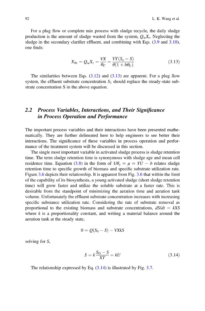
For a plug flow or complete mix process with sludge recycle, the daily sludge
production is the amount of sludge wasted from the system, Q w X r . Neglecting the
sludge in the secondary clarifier effluent, and combining with Eqs. (3.9 and 3.10),
one finds:
X θc ¼ Q w X r ¼
VX
θ C
¼
VY S o À S
ð
Þ
θ 1 þ bθ C
ð
Þ
ð3:13Þ
The similarities between Eqs. (3.12) and (3.13) are apparent. For a plug flow
system, the effluent substrate concentration S 1 should replace the steady-state substrate concentration S in the above equation.
2.2 Process Variables, Interactions, and Their Significance
in Process Operation and Performance
The important process variables and their interactions have been presented mathematically. They are further delineated here to help engineers to see better their
interactions. The significance of these variables in process operation and performance of the treatment system will be discussed in this section.
The single most important variable in activated sludge process is sludge retention
time. The term sludge retention time is synonymous with sludge age and mean cell
residence time. Equation (3.8) in the form of 1/θ c ¼ μ ¼ YU À b relates sludge
retention time to specific growth of biomass and specific substrate utilization rate.
Figure 3.6 depicts their relationship. It is apparent from Fig. 3.6 that within the limit
of the capability of its biosynthesis, a young activated sludge (short sludge retention
time) will grow faster and utilize the soluble substrate at a faster rate. This is
desirable from the standpoint of minimizing the aeration time and aeration tank
volume. Unfortunately the effluent substrate concentration increases with increasing
specific substance utilization rate. Considering the rate of substrate removal as
proportional to the existing biomass and substrate concentrations, dS/dt ¼ kXS
where k is a proportionality constant, and writing a material balance around the
aeration tank at the steady state,
0 ¼ Q S 0 À S
ð
ÞÀVXkS
solving for S,
S ¼ k
S O À S
XT
¼ kU
ð3:14Þ
The relationship expressed by Eq. (3.14) is illustrated by Fig. 3.7.
92
L. K. Wang et al.
production is the amount of sludge wasted from the system, Q w X r . Neglecting the
sludge in the secondary clarifier effluent, and combining with Eqs. (3.9 and 3.10),
one finds:
X θc ¼ Q w X r ¼
VX
θ C
¼
VY S o À S
ð
Þ
θ 1 þ bθ C
ð
Þ
ð3:13Þ
The similarities between Eqs. (3.12) and (3.13) are apparent. For a plug flow
system, the effluent substrate concentration S 1 should replace the steady-state substrate concentration S in the above equation.
2.2 Process Variables, Interactions, and Their Significance
in Process Operation and Performance
The important process variables and their interactions have been presented mathematically. They are further delineated here to help engineers to see better their
interactions. The significance of these variables in process operation and performance of the treatment system will be discussed in this section.
The single most important variable in activated sludge process is sludge retention
time. The term sludge retention time is synonymous with sludge age and mean cell
residence time. Equation (3.8) in the form of 1/θ c ¼ μ ¼ YU À b relates sludge
retention time to specific growth of biomass and specific substrate utilization rate.
Figure 3.6 depicts their relationship. It is apparent from Fig. 3.6 that within the limit
of the capability of its biosynthesis, a young activated sludge (short sludge retention
time) will grow faster and utilize the soluble substrate at a faster rate. This is
desirable from the standpoint of minimizing the aeration time and aeration tank
volume. Unfortunately the effluent substrate concentration increases with increasing
specific substance utilization rate. Considering the rate of substrate removal as
proportional to the existing biomass and substrate concentrations, dS/dt ¼ kXS
where k is a proportionality constant, and writing a material balance around the
aeration tank at the steady state,
0 ¼ Q S 0 À S
ð
ÞÀVXkS
solving for S,
S ¼ k
S O À S
XT
¼ kU
ð3:14Þ
The relationship expressed by Eq. (3.14) is illustrated by Fig. 3.7.
92
L. K. Wang et al.