

12 Magnetic Force Microscopy and Magnetic …
287
12.2 Magnetic Force Microscopy
MFM experimental setups are based on a standard AFM apparatus equipped with a
magnetic tip interacting with the sample through long-range magnetic forces. Some
different MFM experimental approaches have been proposed to detect low-intensity
magnetic fields originated from nanosized samples, e.g., using static or dynamic
detection system, employing ferromagnetic or superparamagnetic tips, involving
or not the application of an external magnetic field, which can be static and/or
alternating.
The most common MFM configuration is based on a two-pass approach, i.e.,
the sample surface is scanned two times [12]. In the first pass, a line is scanned
in tapping mode in order to record the line profile which is used to reconstruct the
sample topography. The line profile is eventually used to scan again the same line
maintaining the tip at fixed distance from the sample surface, namely the lift height
z, which allows the tip to be not sensitive to short range interaction forces, but
only to long range ones such as electrostatic or magnetic forces. During this second
pass, the cantilever is set into oscillation at its first free resonance frequency f 0 (or
at a frequency close to f 0 ) using a bimorph coupled with the cantilever chip. The
presence of a static magnetic field uniform along the direction z perpendicular to
the sample surface modifies equilibrium position of the cantilever without affecting
its oscillation parameters, i.e., the resonance frequency f 0 and the phase shift at
resonance with respect to the excitation θ 0 = −π/2 [12, 14]. Conversely, if the
external magnetic force F is not uniform, the oscillation parameters of the cantilever
depend on the gradient F 1 along z of the component along the same direction of
the force (F z ), i.e., F 1 = ∂ F z /∂z, in correspondence of the equilibrium point of the
cantilever. In particular, the shift in the resonance frequency f 0 and in the phase
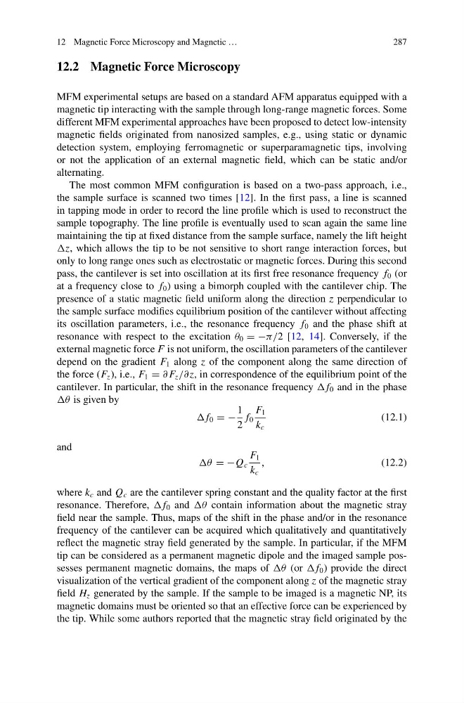
θ is given by
f 0 = −
1
2
f 0
F 1
k c
(12.1)
and
θ = −Q c
F 1
k c
,
(12.2)
where k c and Q c are the cantilever spring constant and the quality factor at the first
resonance. Therefore, f 0 and θ contain information about the magnetic stray
field near the sample. Thus, maps of the shift in the phase and/or in the resonance
frequency of the cantilever can be acquired which qualitatively and quantitatively
reflect the magnetic stray field generated by the sample. In particular, if the MFM
tip can be considered as a permanent magnetic dipole and the imaged sample possesses permanent magnetic domains, the maps of θ (or f 0 ) provide the direct
visualization of the vertical gradient of the component along z of the magnetic stray
field H z generated by the sample. If the sample to be imaged is a magnetic NP, its
magnetic domains must be oriented so that an effective force can be experienced by
the tip. While some authors reported that the magnetic stray field originated by the
287
12.2 Magnetic Force Microscopy
MFM experimental setups are based on a standard AFM apparatus equipped with a
magnetic tip interacting with the sample through long-range magnetic forces. Some
different MFM experimental approaches have been proposed to detect low-intensity
magnetic fields originated from nanosized samples, e.g., using static or dynamic
detection system, employing ferromagnetic or superparamagnetic tips, involving
or not the application of an external magnetic field, which can be static and/or
alternating.
The most common MFM configuration is based on a two-pass approach, i.e.,
the sample surface is scanned two times [12]. In the first pass, a line is scanned
in tapping mode in order to record the line profile which is used to reconstruct the
sample topography. The line profile is eventually used to scan again the same line
maintaining the tip at fixed distance from the sample surface, namely the lift height
z, which allows the tip to be not sensitive to short range interaction forces, but
only to long range ones such as electrostatic or magnetic forces. During this second
pass, the cantilever is set into oscillation at its first free resonance frequency f 0 (or
at a frequency close to f 0 ) using a bimorph coupled with the cantilever chip. The
presence of a static magnetic field uniform along the direction z perpendicular to
the sample surface modifies equilibrium position of the cantilever without affecting
its oscillation parameters, i.e., the resonance frequency f 0 and the phase shift at
resonance with respect to the excitation θ 0 = −π/2 [12, 14]. Conversely, if the
external magnetic force F is not uniform, the oscillation parameters of the cantilever
depend on the gradient F 1 along z of the component along the same direction of
the force (F z ), i.e., F 1 = ∂ F z /∂z, in correspondence of the equilibrium point of the
cantilever. In particular, the shift in the resonance frequency f 0 and in the phase
θ is given by
f 0 = −
1
2
f 0
F 1
k c
(12.1)
and
θ = −Q c
F 1
k c
,
(12.2)
where k c and Q c are the cantilever spring constant and the quality factor at the first
resonance. Therefore, f 0 and θ contain information about the magnetic stray
field near the sample. Thus, maps of the shift in the phase and/or in the resonance
frequency of the cantilever can be acquired which qualitatively and quantitatively
reflect the magnetic stray field generated by the sample. In particular, if the MFM
tip can be considered as a permanent magnetic dipole and the imaged sample possesses permanent magnetic domains, the maps of θ (or f 0 ) provide the direct
visualization of the vertical gradient of the component along z of the magnetic stray
field H z generated by the sample. If the sample to be imaged is a magnetic NP, its
magnetic domains must be oriented so that an effective force can be experienced by
the tip. While some authors reported that the magnetic stray field originated by the