

266
P. Torruella et al.
x j and, thus, it guarantees that under sampling artefacts (Φ domain) are distributed
in a noise-like fashion through the signal in the sparse domain (Ψ ).
The practical application of CS requires of an optimization process to recover the
sparse coefficients from measurements, since the signal acquired is compressed and
the optimal transform Ψ is a priori unknown. To that end, a nonlinear algorithm is
required, able to minimize the number of nonzero coefficients (promoting sparsity)
without compromising the consistency of the measured data. It has been shown that
the minimization can be carried out over the so-called l 1 -norm [35]
c =
i |c i |.
11.2.1.2 Compressed Sensing in Electron Tomography (CS-ET)
CS-ET can be formulated from two different equivalent perspectives: (i) being
p the
projection image (sinogram) and Φ the real space projection operator in the frame of
a discretized Radon transform or (ii) applying the central slice theorem in the frame
of a discretized Fourier transform (FT). This second approach sets
p as the FT of
the projection data (i.e. discrete radial samples of the object in the Fourier space),
and Φ as a discrete Fourier operator. Then, the under sampling artefacts (already
discussed in the introduction) that arise from an uncomplete radial sampling of the
Fourier space can be minimized through the effective application of a CS-based
reconstruction algorithm.
The sparsity of the signals recorded (necessary condition for the application of CS)
must be promoted through a certain transform Ψ . Several possibilities of transforms
are described in the literature, depending on the sample nature and projection images
information content (acquisition mode). The most common choice is a combination
of sparse transform in the image domain itself (Ψ = I identity transform) and the
spatial gradient domain (Ψ = spatial finite-differences transform). The sparsity is
then promoted by minimizing the l 1 -norm in both spaces (being called the TV-norm
in the spatial gradient space). This is a convex optimization problem that can be
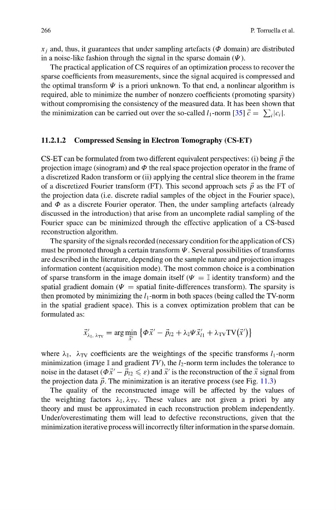
formulated as:
x
λ I , λ TV
= arg min
x
Φ
x
− −
p l2 + λ I Ψ
x
l1 + λ TV TV
x
where λ I , λ TV coefficients are the weightings of the specific transforms l 1 -norm
minimization (image I and gradient TV ), the l 2 -norm term includes the tolerance to
noise in the dataset (Φ
x
− −
p l2 ε) and
x
is the reconstruction of the
x signal from
the projection data
p. The minimization is an iterative process (see Fig. 11.3)
The quality of the reconstructed image will be affected by the values of
the weighting factors λ I , λ TV . These values are not given a priori by any
theory and must be approximated in each reconstruction problem independently.
Under/overestimating them will lead to defective reconstructions, given that the
minimization iterative process will incorrectly filter information in the sparse domain.
P. Torruella et al.
x j and, thus, it guarantees that under sampling artefacts (Φ domain) are distributed
in a noise-like fashion through the signal in the sparse domain (Ψ ).
The practical application of CS requires of an optimization process to recover the
sparse coefficients from measurements, since the signal acquired is compressed and
the optimal transform Ψ is a priori unknown. To that end, a nonlinear algorithm is
required, able to minimize the number of nonzero coefficients (promoting sparsity)
without compromising the consistency of the measured data. It has been shown that
the minimization can be carried out over the so-called l 1 -norm [35]
c =
i |c i |.
11.2.1.2 Compressed Sensing in Electron Tomography (CS-ET)
CS-ET can be formulated from two different equivalent perspectives: (i) being
p the
projection image (sinogram) and Φ the real space projection operator in the frame of
a discretized Radon transform or (ii) applying the central slice theorem in the frame
of a discretized Fourier transform (FT). This second approach sets
p as the FT of
the projection data (i.e. discrete radial samples of the object in the Fourier space),
and Φ as a discrete Fourier operator. Then, the under sampling artefacts (already
discussed in the introduction) that arise from an uncomplete radial sampling of the
Fourier space can be minimized through the effective application of a CS-based
reconstruction algorithm.
The sparsity of the signals recorded (necessary condition for the application of CS)
must be promoted through a certain transform Ψ . Several possibilities of transforms
are described in the literature, depending on the sample nature and projection images
information content (acquisition mode). The most common choice is a combination
of sparse transform in the image domain itself (Ψ = I identity transform) and the
spatial gradient domain (Ψ = spatial finite-differences transform). The sparsity is
then promoted by minimizing the l 1 -norm in both spaces (being called the TV-norm
in the spatial gradient space). This is a convex optimization problem that can be
formulated as:
x
λ I , λ TV
= arg min
x
Φ
x
− −
p l2 + λ I Ψ
x
l1 + λ TV TV
x
where λ I , λ TV coefficients are the weightings of the specific transforms l 1 -norm
minimization (image I and gradient TV ), the l 2 -norm term includes the tolerance to
noise in the dataset (Φ
x
− −
p l2 ε) and
x
is the reconstruction of the
x signal from
the projection data
p. The minimization is an iterative process (see Fig. 11.3)
The quality of the reconstructed image will be affected by the values of
the weighting factors λ I , λ TV . These values are not given a priori by any
theory and must be approximated in each reconstruction problem independently.
Under/overestimating them will lead to defective reconstructions, given that the
minimization iterative process will incorrectly filter information in the sparse domain.