

of each molecule. We seek the number p of complexions where w 0 [number of]
molecules have kinetic energy 0, w 1 molecules have kinetic energy E, w 2 have kinetic
energy 2E, upto the w p which have kinetic energy pε. We said, earlier, that given how
many molecules have kinetic energy 0, how many have kinetic energy E, etc., this
distribution among the molecules specifies the number of P of complexions for that
distribution; in other words, it determines the likelihood of that state distribution.
Dividing the number P by the number of all possible complexions, we get the
probability of the state distribution. Boltzmann actually never performs this division.
It is done later by Max Planck (1901).
Since a distribution of states does not determine kinetic energies exactly, the goal
is to describe the state distribution by writing as many zeros as molecules with zero
kinetic energy (w 0 ), w 1 ones for those with kinetic energy E, etc. All these zeros,
ones, etc. are the elements defining the state distribution. It is now immediately clear
that the number P for each state distribution is exactly the same as the number of
permutations of which the elements of the state distribution are capable and that is
why the number P is the desired measure of the permutability of the corresponding
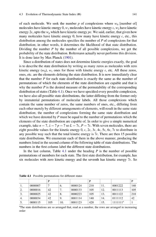
distribution of states (Table 4.1). Once we have specified every possible complexion,
we have also all possible state distributions, the latter differing from the former only
by immaterial permutations of molecular labels. All those complexions which
contain the same number of zeros, the same numbers of ones, etc., differing from
each other merely by different arrangements of elements, will result in the same state
distribution; the number of complexions forming the same state distribution and
which we have denoted by P must be equal to the number of permutations which the
elements of the state distribution are capable of. In order to give a simple numerical
example, take n ¼ 7, λ ¼ 7 p ¼ 7 so L ¼ 7E, P ¼ 7E. With seven molecules, there are
eight possible values for the kinetic energy 0, E, 2E, 3E, 4E, 5E, 6E, 7E to distribute in
any possible way such that the total kinetic energy is 7E. There are then 15 possible
state distributions. We enumerate each of them in the above manner, producing the
numbers listed in the second column of the following table of state distributions. The
numbers in the first column label the different state distributions.
In the last column, Table 4.1 under the heading P is the number of possible
permutations of members for each state. The first state distribution, for example, has
six molecules with zero kinetic energy and the seventh has kinetic energy 7E. So
Table 4.1 Possible permutations for different states
P
P
P
1.
0000007
7
6.
0000124
210
11.
0001222
140
2.
0000016
42
7.
0000133
105
12.
0011113
105
3.
0000025
42
8.
0000223
105
13.
0011122
210
4.
0000034
42
9.
0001114
140
14.
0111112
42
5.
0000115
105
10.
0001123
420
15.
1111111
a
1
a The state distributions are so arranged that, read as a number, the rows are arranged in increasing
order
4.3 Evolution of Thermodynamic State Index (Φ)
141
molecules have kinetic energy 0, w 1 molecules have kinetic energy E, w 2 have kinetic
energy 2E, upto the w p which have kinetic energy pε. We said, earlier, that given how
many molecules have kinetic energy 0, how many have kinetic energy E, etc., this
distribution among the molecules specifies the number of P of complexions for that
distribution; in other words, it determines the likelihood of that state distribution.
Dividing the number P by the number of all possible complexions, we get the
probability of the state distribution. Boltzmann actually never performs this division.
It is done later by Max Planck (1901).
Since a distribution of states does not determine kinetic energies exactly, the goal
is to describe the state distribution by writing as many zeros as molecules with zero
kinetic energy (w 0 ), w 1 ones for those with kinetic energy E, etc. All these zeros,
ones, etc. are the elements defining the state distribution. It is now immediately clear
that the number P for each state distribution is exactly the same as the number of
permutations of which the elements of the state distribution are capable and that is
why the number P is the desired measure of the permutability of the corresponding
distribution of states (Table 4.1). Once we have specified every possible complexion,
we have also all possible state distributions, the latter differing from the former only
by immaterial permutations of molecular labels. All those complexions which
contain the same number of zeros, the same numbers of ones, etc., differing from
each other merely by different arrangements of elements, will result in the same state
distribution; the number of complexions forming the same state distribution and
which we have denoted by P must be equal to the number of permutations which the
elements of the state distribution are capable of. In order to give a simple numerical
example, take n ¼ 7, λ ¼ 7 p ¼ 7 so L ¼ 7E, P ¼ 7E. With seven molecules, there are
eight possible values for the kinetic energy 0, E, 2E, 3E, 4E, 5E, 6E, 7E to distribute in
any possible way such that the total kinetic energy is 7E. There are then 15 possible
state distributions. We enumerate each of them in the above manner, producing the
numbers listed in the second column of the following table of state distributions. The
numbers in the first column label the different state distributions.
In the last column, Table 4.1 under the heading P is the number of possible
permutations of members for each state. The first state distribution, for example, has
six molecules with zero kinetic energy and the seventh has kinetic energy 7E. So
Table 4.1 Possible permutations for different states
P
P
P
1.
0000007
7
6.
0000124
210
11.
0001222
140
2.
0000016
42
7.
0000133
105
12.
0011113
105
3.
0000025
42
8.
0000223
105
13.
0011122
210
4.
0000034
42
9.
0001114
140
14.
0111112
42
5.
0000115
105
10.
0001123
420
15.
1111111
a
1
a The state distributions are so arranged that, read as a number, the rows are arranged in increasing
order
4.3 Evolution of Thermodynamic State Index (Φ)
141