

518
13 Fiber Optic Communication Networks
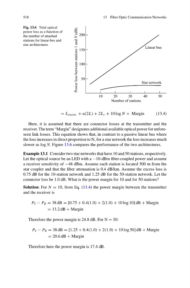
Fig. 13.6 Total optical
power loss as a function of
the number of attached
stations for linear-bus and
star architectures
= L excess + α(2L) + 2L c + 10 log N + Margin
(13.4)
Here, it is assumed that there are connector losses at the transmitter and the
receiver. The term “Margin” designates additional available optical power for unforeseen link losses. This equation shows that, in contrast to a passive linear bus where
the loss increases in direct proportion to N, for a star network the loss increases much
slower as log N. Figure 13.6 compares the performance of the two architectures.
Example 13.1 Consider two star networks that have 10 and 50 stations, respectively.
Let the optical source be an LED with a −10-dBm fiber-coupled power and assume
a receiver sensitivity of −48 dBm. Assume each station is located 500 m from the
star coupler and that the fiber attenuation is 0.4 dB/km. Assume the excess loss is
0.75 dB for the 10-station network and 1.25 dB for the 50-station network. Let the
connector loss be 1.0 dB. What is the power margin for 10 and for 50 stations?
Solution: For N = 10, from Eq. (13.4) the power margin between the transmitter
and the receiver is
P S − P R = 38 dB = [0.75 + 0.4(1.0) + 2(1.0) + 10 log 10] dB + Margin
= 13.2 dB + Margin
Therefore the power margin is 24.8 dB. For N = 50:
P S − P R = 38 dB = [1.25 + 0.4(1.0) + 2(1.0) + 10 log 50] dB + Margin
= 20.6 dB + Margin
Therefore here the power margin is 17.4 dB.
13 Fiber Optic Communication Networks
Fig. 13.6 Total optical
power loss as a function of
the number of attached
stations for linear-bus and
star architectures
= L excess + α(2L) + 2L c + 10 log N + Margin
(13.4)
Here, it is assumed that there are connector losses at the transmitter and the
receiver. The term “Margin” designates additional available optical power for unforeseen link losses. This equation shows that, in contrast to a passive linear bus where
the loss increases in direct proportion to N, for a star network the loss increases much
slower as log N. Figure 13.6 compares the performance of the two architectures.
Example 13.1 Consider two star networks that have 10 and 50 stations, respectively.
Let the optical source be an LED with a −10-dBm fiber-coupled power and assume
a receiver sensitivity of −48 dBm. Assume each station is located 500 m from the
star coupler and that the fiber attenuation is 0.4 dB/km. Assume the excess loss is
0.75 dB for the 10-station network and 1.25 dB for the 50-station network. Let the
connector loss be 1.0 dB. What is the power margin for 10 and for 50 stations?
Solution: For N = 10, from Eq. (13.4) the power margin between the transmitter
and the receiver is
P S − P R = 38 dB = [0.75 + 0.4(1.0) + 2(1.0) + 10 log 10] dB + Margin
= 13.2 dB + Margin
Therefore the power margin is 24.8 dB. For N = 50:
P S − P R = 38 dB = [1.25 + 0.4(1.0) + 2(1.0) + 10 log 50] dB + Margin
= 20.6 dB + Margin
Therefore here the power margin is 17.4 dB.