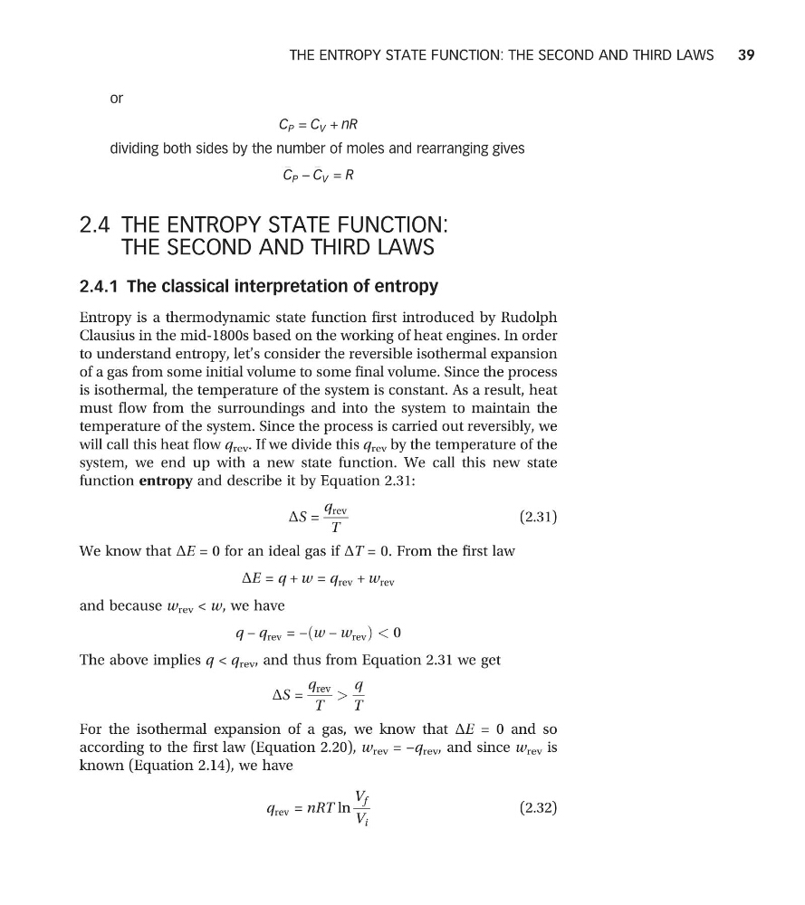
or
C P = C V + nR
dividing both sides by the number of moles and rearranging gives
C P −
C V = R
2.4 THE ENTROPY STATE FUNCTION:
THE SECOND AND THIRD LAWS
2.4.1 The classical interpretation of entropy
Entropy is a thermodynamic state function first introduced by Rudolph
Clausius in the mid-1800s based on the working of heat engines. In order
to understand entropy, let’s consider the reversible isothermal expansion
of a gas from some initial volume to some final volume. Since the process
is isothermal, the temperature of the system is constant. As a result, heat
must flow from the surroundings and into the system to maintain the
temperature of the system. Since the process is carried out reversibly, we
will call this heat flow q rev . If we divide this q rev by the temperature of the
system, we end up with a new state function. We call this new state
function entropy and describe it by Equation 2.31:
ΔS =
q rev
T
(2.31)
We know that ΔE = 0 for an ideal gas if ΔT = 0. From the first law
ΔE = q + w = q rev + w rev
and because w rev < w, we have
q − q rev = − w − w rev
ð
Þ< 0
The above implies q < q rev , and thus from Equation 2.31 we get
ΔS =
q rev
T
>
q
T
For the isothermal expansion of a gas, we know that ΔE = 0 and so
according to the first law (Equation 2.20), w rev = −q rev , and since w rev is
known (Equation 2.14), we have
q rev = nRT ln
V f
V i
(2.32)
THE ENTROPY STATE FUNCTION: THE SECOND AND THIRD LAWS
39