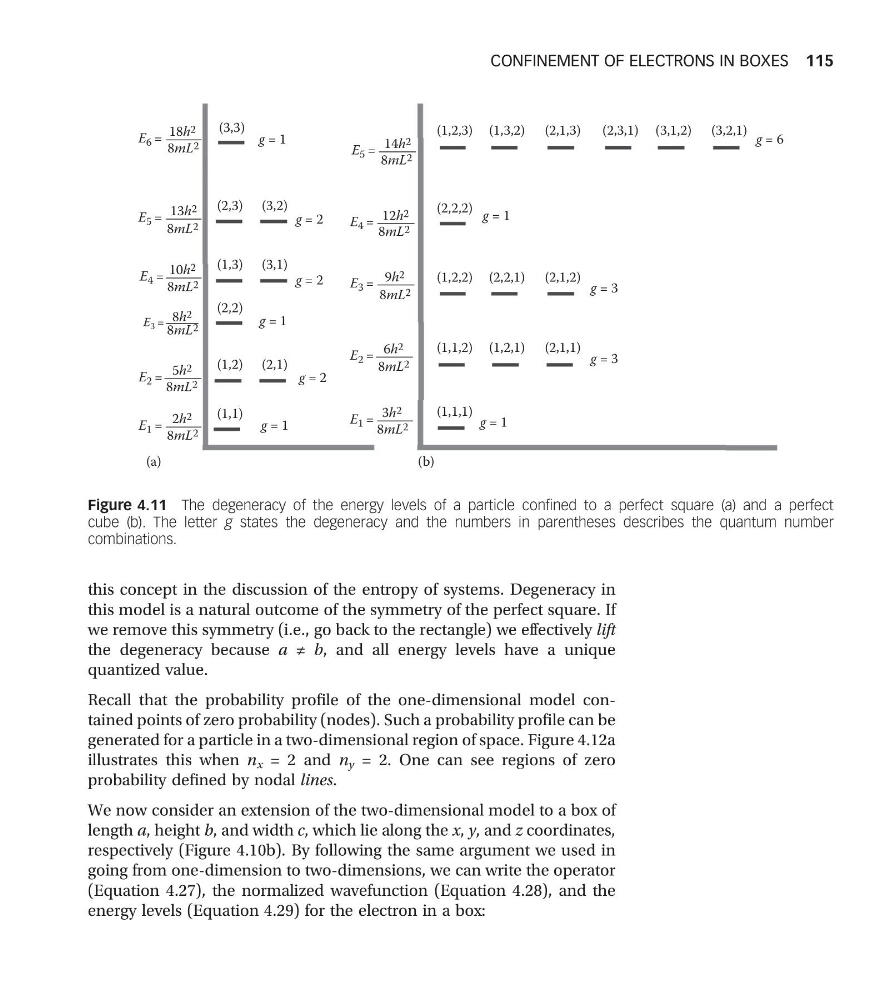
this concept in the discussion of the entropy of systems. Degeneracy in
this model is a natural outcome of the symmetry of the perfect square. If
we remove this symmetry (i.e., go back to the rectangle) we effectively lift
the degeneracy because a ≠ b, and all energy levels have a unique
quantized value.
Recall that the probability profile of the one-dimensional model contained points of zero probability (nodes). Such a probability profile can be
generated for a particle in a two-dimensional region of space. Figure 4.12a
illustrates this when n x = 2 and n y = 2. One can see regions of zero
probability defined by nodal lines.
We now consider an extension of the two-dimensional model to a box of
length a, height b, and width c, which lie along the x, y, and z coordinates,
respectively (Figure 4.10b). By following the same argument we used in
going from one-dimension to two-dimensions, we can write the operator
(Equation 4.27), the normalized wavefunction (Equation 4.28), and the
energy levels (Equation 4.29) for the electron in a box:
E 6 = 18h 2
8mL 2
E 5 = 14h 2
8mL 2
E 4 = 12h 2
8mL 2
E 5 = 13h 2
8mL 2
E 4 = 10h 2
8mL 2
E 3 = 8h 2
8mL 2
E 2 = 5h 2
8mL 2
E 3 = 9h 2
8mL 2
E 2 = 6h 2
8mL 2
E 1 = 3h 2
8mL 2
E 1 = 2h 2
8mL 2
(3,3)
(1,2,3)
(2,2,2)
(1,3,2) (2,1,3)
(1,2,2) (2,2,1) (2,1,2)
(1,1,2)
(1,1,1)
(1,2,1) (2,1,1)
(2,3,1) (3,1,2) (3,2,1)
(2,3)
g = 1
g = 6
g = 1
g = 3
g = 3
g = 1
g = 2
g = 2
g = 1
g = 2
g = 1
(3,2)
(1,3)
(2,2)
(3,1)
(1,2)
(1,1)
(2,1)
(a)
(b)
Figure 4.11 The degeneracy of the energy levels of a particle confined to a perfect square (a) and a perfect
cube (b). The letter g states the degeneracy and the numbers in parentheses describes the quantum number
combinations.
CONFINEMENT OF ELECTRONS IN BOXES 115