

Equation 4.18 shows that the electron can only have discrete energy values
that are dictated by the value of n. For example, the ground state energy of
the electron will be given when n = 1. This energy according to Equation
4.18 is h
2 /8mL
2 . Figure 4.5 summarizes the allowed energies as a function
of n. The spacing between the energy levels increase as n increases. Also
sketched in Figure 4.5 are the wavefunctions and the wavefunctions
squared. Interpretation of the wavefunction squared allows us to examine
the probability profile of the electron along the x-direction.
In this one-dimensional electron on a line segment model, the electron
does not exist as a discrete particle moving along the line. Rather, it resembles a standing wave whose exact form depends on the value of n. The
standing waves can be viewed as a cloud of electron density with regions of
high and low electron probability. Regions where the wavefunction equals
zero correspond to a zero electron probability and are known as nodes.
Because we interpret the wavefunction in terms of probabilities, we can
determine the likelihood of finding the electron in a given region of space.
We illustrate this in Example 4.5, where we see that the probability of
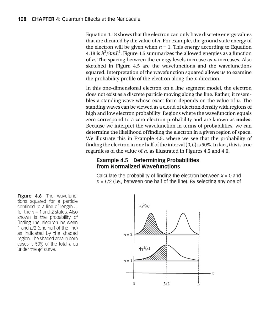
finding the electron in one half of the interval (0,L) is 50%. In fact, this is true
regardless of the value of n, as illustrated in Figures 4.5 and 4.6.
Example 4.5 Determining Probabilities
from Normalized Wavefunctions
Calculate the probability of finding the electron between x = 0 and
x = L/2 (i.e., between one half of the line). By selecting any one of
ψ 2
2 (x)
ψ 1
2 (x)
n = 2
n = 1
L/2
L
x
0
Figure 4.6 The wavefunctions squared for a particle
confined to a line of length L,
for the n = 1 and 2 states. Also
shown is the probability of
finding the electron between
1 and L/2 (one half of the line)
as indicated by the shaded
region. The shaded area in both
cases is 50% of the total area
under the ψ
2 curve.
CHAPTER 4: Quantum Effects at the Nanoscale
108
that are dictated by the value of n. For example, the ground state energy of
the electron will be given when n = 1. This energy according to Equation
4.18 is h
2 /8mL
2 . Figure 4.5 summarizes the allowed energies as a function
of n. The spacing between the energy levels increase as n increases. Also
sketched in Figure 4.5 are the wavefunctions and the wavefunctions
squared. Interpretation of the wavefunction squared allows us to examine
the probability profile of the electron along the x-direction.
In this one-dimensional electron on a line segment model, the electron
does not exist as a discrete particle moving along the line. Rather, it resembles a standing wave whose exact form depends on the value of n. The
standing waves can be viewed as a cloud of electron density with regions of
high and low electron probability. Regions where the wavefunction equals
zero correspond to a zero electron probability and are known as nodes.
Because we interpret the wavefunction in terms of probabilities, we can
determine the likelihood of finding the electron in a given region of space.
We illustrate this in Example 4.5, where we see that the probability of
finding the electron in one half of the interval (0,L) is 50%. In fact, this is true
regardless of the value of n, as illustrated in Figures 4.5 and 4.6.
Example 4.5 Determining Probabilities
from Normalized Wavefunctions
Calculate the probability of finding the electron between x = 0 and
x = L/2 (i.e., between one half of the line). By selecting any one of
ψ 2
2 (x)
ψ 1
2 (x)
n = 2
n = 1
L/2
L
x
0
Figure 4.6 The wavefunctions squared for a particle
confined to a line of length L,
for the n = 1 and 2 states. Also
shown is the probability of
finding the electron between
1 and L/2 (one half of the line)
as indicated by the shaded
region. The shaded area in both
cases is 50% of the total area
under the ψ
2 curve.
CHAPTER 4: Quantum Effects at the Nanoscale
108