

V 1 ¼ dN
g
pop
ð7:2Þ
which correspond to the straight lines in logarithmic scale. For this purpose, we can
use the method presented in Chap. 2 and Eq. (2.3), if we substitute y by ln a and
ln V 1 for (7.1) and (7.2), respectively. Accordingly, the variable t has to be substituted by ln N pop ; the parameters c have to be substituted by v and g for (7.1) and
(7.2), respectively; the parameter b—by ln r and ln d for (7.1) and (7.2), respectively. Then we can calculate the values y j and t j with the use of data set presented
in Table 7.1 and the linear regression (e.g., formulas (2.6)–(2.9)). The results of
calculations are shown in Table 7.2 for different amount of elements in the data sets
(n = 13 for complete data set and n = 11 for the data set without figures for China
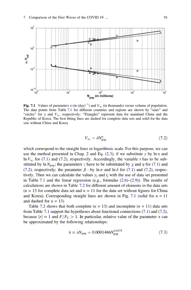
and Korea). Corresponding straight lines are shown in Fig. 7.1 (solid for n = 11
and dashed for n = 13)
Table 7.2 shows that both complete (n = 13) and incomplete (n = 11) data sets
from Table 7.1 support the hypotheses about functional connections (7.1) and (7.2),
because r
j j % 1 and F=F C [ 1. In particular, relative value of the parameter a can
be approximated by the following relationships:
a aN pop ¼ 0:0001466N
0:0375
pop
ð7:3Þ
Fig. 7.1 Values of parameters a (in (day)
−1
) and V 1 (in thousands) versus volume of population.
The data points from Table 7.1 for different countries and regions are shown by “stars” and
“circles” for a and V 1 , respectively: “Triangles” represent data for mainland China and the
Republic of Korea. The best fitting lines are dashed for complete data sets and solid for the data
sets without China and Korea
7 Comparison of the First Waves of the COVID-19 …
91
g
pop
ð7:2Þ
which correspond to the straight lines in logarithmic scale. For this purpose, we can
use the method presented in Chap. 2 and Eq. (2.3), if we substitute y by ln a and
ln V 1 for (7.1) and (7.2), respectively. Accordingly, the variable t has to be substituted by ln N pop ; the parameters c have to be substituted by v and g for (7.1) and
(7.2), respectively; the parameter b—by ln r and ln d for (7.1) and (7.2), respectively. Then we can calculate the values y j and t j with the use of data set presented
in Table 7.1 and the linear regression (e.g., formulas (2.6)–(2.9)). The results of
calculations are shown in Table 7.2 for different amount of elements in the data sets
(n = 13 for complete data set and n = 11 for the data set without figures for China
and Korea). Corresponding straight lines are shown in Fig. 7.1 (solid for n = 11
and dashed for n = 13)
Table 7.2 shows that both complete (n = 13) and incomplete (n = 11) data sets
from Table 7.1 support the hypotheses about functional connections (7.1) and (7.2),
because r
j j % 1 and F=F C [ 1. In particular, relative value of the parameter a can
be approximated by the following relationships:
a aN pop ¼ 0:0001466N
0:0375
pop
ð7:3Þ
Fig. 7.1 Values of parameters a (in (day)
−1
) and V 1 (in thousands) versus volume of population.
The data points from Table 7.1 for different countries and regions are shown by “stars” and
“circles” for a and V 1 , respectively: “Triangles” represent data for mainland China and the
Republic of Korea. The best fitting lines are dashed for complete data sets and solid for the data
sets without China and Korea
7 Comparison of the First Waves of the COVID-19 …
91