

4.3 Flux Flow State
63
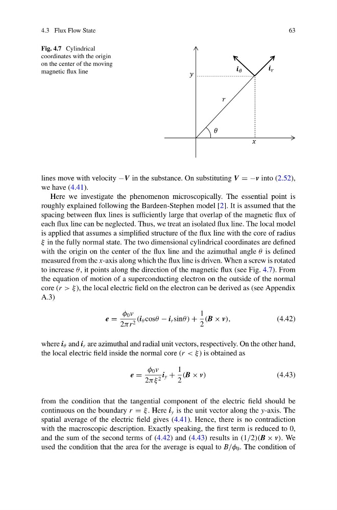
Fig. 4.7 Cylindrical
coordinates with the origin
on the center of the moving
magnetic flux line
lines move with velocity −V in the substance. On substituting V = −v into (2.52),
we have (4.41).
Here we investigate the phenomenon microscopically. The essential point is
roughly explained following the Bardeen-Stephen model [2]. It is assumed that the
spacing between flux lines is sufficiently large that overlap of the magnetic flux of
each flux line can be neglected. Thus, we treat an isolated flux line. The local model
is applied that assumes a simplified structure of the flux line with the core of radius
ξ in the fully normal state. The two dimensional cylindrical coordinates are defined
with the origin on the center of the flux line and the azimuthal angle θ is defined
measured from the x-axis along which the flux line is driven. When a screw is rotated
to increase θ , it points along the direction of the magnetic flux (see Fig. 4.7). From
the equation of motion of a superconducting electron on the outside of the normal
core (r > ξ), the local electric field on the electron can be derived as (see Appendix
A.3)
e =
φ 0 v
2π r 2 (i θ cosθ − i r sinθ ) +
1
2
(B × v),
(4.42)
where i θ and i r are azimuthal and radial unit vectors, respectively. On the other hand,
the local electric field inside the normal core (r < ξ) is obtained as
e =
φ 0 v
2πξ 2 i y +
1
2
(B × v)
(4.43)
from the condition that the tangential component of the electric field should be
continuous on the boundary r = ξ . Here i y is the unit vector along the y-axis. The
spatial average of the electric field gives (4.41). Hence, there is no contradiction
with the macroscopic description. Exactly speaking, the first term is reduced to 0,
and the sum of the second terms of (4.42) and (4.43) results in (1/2)(B × v). We
used the condition that the area for the average is equal to B/φ 0 . The condition of
63
Fig. 4.7 Cylindrical
coordinates with the origin
on the center of the moving
magnetic flux line
lines move with velocity −V in the substance. On substituting V = −v into (2.52),
we have (4.41).
Here we investigate the phenomenon microscopically. The essential point is
roughly explained following the Bardeen-Stephen model [2]. It is assumed that the
spacing between flux lines is sufficiently large that overlap of the magnetic flux of
each flux line can be neglected. Thus, we treat an isolated flux line. The local model
is applied that assumes a simplified structure of the flux line with the core of radius
ξ in the fully normal state. The two dimensional cylindrical coordinates are defined
with the origin on the center of the flux line and the azimuthal angle θ is defined
measured from the x-axis along which the flux line is driven. When a screw is rotated
to increase θ , it points along the direction of the magnetic flux (see Fig. 4.7). From
the equation of motion of a superconducting electron on the outside of the normal
core (r > ξ), the local electric field on the electron can be derived as (see Appendix
A.3)
e =
φ 0 v
2π r 2 (i θ cosθ − i r sinθ ) +
1
2
(B × v),
(4.42)
where i θ and i r are azimuthal and radial unit vectors, respectively. On the other hand,
the local electric field inside the normal core (r < ξ) is obtained as
e =
φ 0 v
2πξ 2 i y +
1
2
(B × v)
(4.43)
from the condition that the tangential component of the electric field should be
continuous on the boundary r = ξ . Here i y is the unit vector along the y-axis. The
spatial average of the electric field gives (4.41). Hence, there is no contradiction
with the macroscopic description. Exactly speaking, the first term is reduced to 0,
and the sum of the second terms of (4.42) and (4.43) results in (1/2)(B × v). We
used the condition that the area for the average is equal to B/φ 0 . The condition of