

2.4 Electromagnetic Phenomena Varying with Time
25
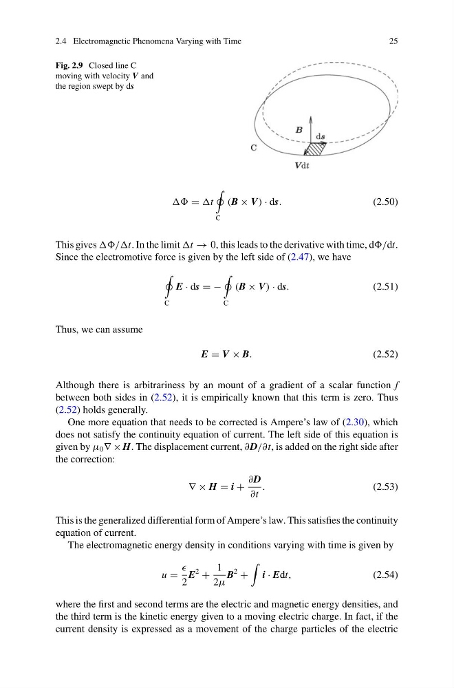
Fig. 2.9 Closed line C
moving with velocity V and
the region swept by ds
= t
C
(B × V) · ds.
(2.50)
This gives //t. In the limit t → 0, this leads to the derivative with time, d/dt.
Since the electromotive force is given by the left side of (2.47), we have
C
E · ds = −
C
(B × V) · ds.
(2.51)
Thus, we can assume
E = V × B.
(2.52)
Although there is arbitrariness by an mount of a gradient of a scalar function f
between both sides in (2.52), it is empirically known that this term is zero. Thus
(2.52) holds generally.
One more equation that needs to be corrected is Ampere’s law of (2.30), which
does not satisfy the continuity equation of current. The left side of this equation is
given by μ 0 ∇ × H. The displacement current, ∂D/∂t, is added on the right side after
the correction:
∇ × H = i +
∂D
∂t
.
(2.53)
This is the generalized differential form of Ampere’s law. This satisfies the continuity
equation of current.
The electromagnetic energy density in conditions varying with time is given by
u =
2
E
2
+
1
2μ
B
2
+
i · Edt,
(2.54)
where the first and second terms are the electric and magnetic energy densities, and
the third term is the kinetic energy given to a moving electric charge. In fact, if the
current density is expressed as a movement of the charge particles of the electric
25
Fig. 2.9 Closed line C
moving with velocity V and
the region swept by ds
= t
C
(B × V) · ds.
(2.50)
This gives //t. In the limit t → 0, this leads to the derivative with time, d/dt.
Since the electromotive force is given by the left side of (2.47), we have
C
E · ds = −
C
(B × V) · ds.
(2.51)
Thus, we can assume
E = V × B.
(2.52)
Although there is arbitrariness by an mount of a gradient of a scalar function f
between both sides in (2.52), it is empirically known that this term is zero. Thus
(2.52) holds generally.
One more equation that needs to be corrected is Ampere’s law of (2.30), which
does not satisfy the continuity equation of current. The left side of this equation is
given by μ 0 ∇ × H. The displacement current, ∂D/∂t, is added on the right side after
the correction:
∇ × H = i +
∂D
∂t
.
(2.53)
This is the generalized differential form of Ampere’s law. This satisfies the continuity
equation of current.
The electromagnetic energy density in conditions varying with time is given by
u =
2
E
2
+
1
2μ
B
2
+
i · Edt,
(2.54)
where the first and second terms are the electric and magnetic energy densities, and
the third term is the kinetic energy given to a moving electric charge. In fact, if the
current density is expressed as a movement of the charge particles of the electric