

12
2 Basic Electromagnetism
where 0
= 8.8542 × 10
−12 C
2
/Nm
2
is the permittivity of vacuum and the above
integration is carried out with respect to r
. Equation (2.2) is called Coulomb’s law.
In (2.2) the electric field contributed from a point-like charge, ρdV
, is summed up;
r − r
/
r − r
3 is a vector directed from the electric charge at r
to the observation
point at r and its magnitude is the inverse of the square of the distance between the
two points. When the electric field is integrated on a closed surface S, the following
relationship holds:
S
E · dS =
1
0
V
ρ(r)dV ,
(2.3)
where V is the space surrounded by S and the elementary surface vector dS is directed
outwards. This is called Gauss’ law. While Coulomb’s law describes the local electric
field produced by electric charge, Gauss’ law gives the global relationship between
electric field and electric charge.
We consider the case where electric charge Q is placed on the origin (r = 0). If
S is a spherical surface of radius r with its center on the origin, the electric field E
is parallel to the elementary surface vector dS and its magnitude is a constant value
on the surface on the left side of (2.3). Hence, the left side is given by 4π r
2 E. Since
the right side is Q// 0 , we have
E =
Q
4ππ 0 r 2 .
(2.4)
This is nothing else than the relationship given by (2.2). That is, Coulomb’s law and
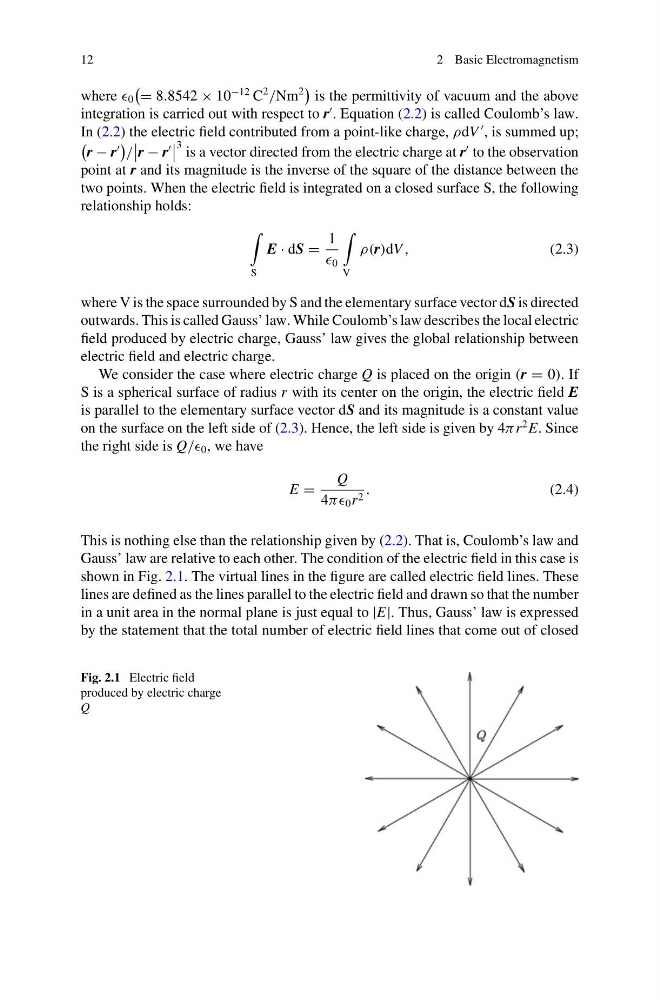
Gauss’ law are relative to each other. The condition of the electric field in this case is
shown in Fig. 2.1. The virtual lines in the figure are called electric field lines. These
lines are defined as the lines parallel to the electric field and drawn so that the number
in a unit area in the normal plane is just equal to |E|. Thus, Gauss’ law is expressed
by the statement that the total number of electric field lines that come out of closed
Fig. 2.1 Electric field
produced by electric charge
Q
2 Basic Electromagnetism
where 0
= 8.8542 × 10
−12 C
2
/Nm
2
is the permittivity of vacuum and the above
integration is carried out with respect to r
. Equation (2.2) is called Coulomb’s law.
In (2.2) the electric field contributed from a point-like charge, ρdV
, is summed up;
r − r
/
r − r
3 is a vector directed from the electric charge at r
to the observation
point at r and its magnitude is the inverse of the square of the distance between the
two points. When the electric field is integrated on a closed surface S, the following
relationship holds:
S
E · dS =
1
0
V
ρ(r)dV ,
(2.3)
where V is the space surrounded by S and the elementary surface vector dS is directed
outwards. This is called Gauss’ law. While Coulomb’s law describes the local electric
field produced by electric charge, Gauss’ law gives the global relationship between
electric field and electric charge.
We consider the case where electric charge Q is placed on the origin (r = 0). If
S is a spherical surface of radius r with its center on the origin, the electric field E
is parallel to the elementary surface vector dS and its magnitude is a constant value
on the surface on the left side of (2.3). Hence, the left side is given by 4π r
2 E. Since
the right side is Q// 0 , we have
E =
Q
4ππ 0 r 2 .
(2.4)
This is nothing else than the relationship given by (2.2). That is, Coulomb’s law and
Gauss’ law are relative to each other. The condition of the electric field in this case is
shown in Fig. 2.1. The virtual lines in the figure are called electric field lines. These
lines are defined as the lines parallel to the electric field and drawn so that the number
in a unit area in the normal plane is just equal to |E|. Thus, Gauss’ law is expressed
by the statement that the total number of electric field lines that come out of closed
Fig. 2.1 Electric field
produced by electric charge
Q