

Electrostatics of the Nanowires with Radial …
87
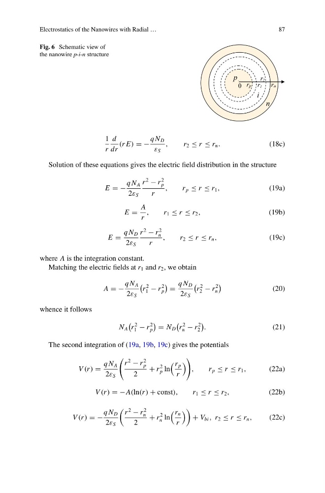
Fig. 6 Schematic view of
the nanowire p-i-n structure
0
r n
p
n
r p r 1
r 2
i
1
r
d
dr
(r E) = −
q N D
ε S
,
r 2 ≤ r ≤ r n .
(18c)
Solution of these equations gives the electric field distribution in the structure
E = −
q N A
2ε S
r
2
− r
2
p
r
,
r p ≤ r ≤ r 1 ,
(19a)
E =
A
r
,
r 1 ≤ r ≤ r 2 ,
(19b)
E =
q N D
2ε S
r
2
− r
2
n
r
,
r 2 ≤ r ≤ r n ,
(19c)
where A is the integration constant.
Matching the electric fields at r 1 and r 2 , we obtain
A = −
q N A
2ε S
r
2
1 − r
2
p
=
q N D
2ε S
r
2
2 − r
2
n
(20)
whence it follows
N A
r
2
1 − r
2
p
= N D
r
2
n − r
2
2
.
(21)
The second integration of (19a, 19b, 19c) gives the potentials
V (r ) =
q N A
2ε S
r
2
− r
2
p
2
+ r
2
p ln
r p
r
,
r p ≤ r ≤ r 1 ,
(22a)
V (r ) = −A(ln(r ) + const),
r 1 ≤ r ≤ r 2 ,
(22b)
V (r ) = −
q N D
2ε S
r
2
− r
2
n
2
+ r
2
n ln
r n
r
+ V bi , r 2 ≤ r ≤ r n ,
(22c)
87
Fig. 6 Schematic view of
the nanowire p-i-n structure
0
r n
p
n
r p r 1
r 2
i
1
r
d
dr
(r E) = −
q N D
ε S
,
r 2 ≤ r ≤ r n .
(18c)
Solution of these equations gives the electric field distribution in the structure
E = −
q N A
2ε S
r
2
− r
2
p
r
,
r p ≤ r ≤ r 1 ,
(19a)
E =
A
r
,
r 1 ≤ r ≤ r 2 ,
(19b)
E =
q N D
2ε S
r
2
− r
2
n
r
,
r 2 ≤ r ≤ r n ,
(19c)
where A is the integration constant.
Matching the electric fields at r 1 and r 2 , we obtain
A = −
q N A
2ε S
r
2
1 − r
2
p
=
q N D
2ε S
r
2
2 − r
2
n
(20)
whence it follows
N A
r
2
1 − r
2
p
= N D
r
2
n − r
2
2
.
(21)
The second integration of (19a, 19b, 19c) gives the potentials
V (r ) =
q N A
2ε S
r
2
− r
2
p
2
+ r
2
p ln
r p
r
,
r p ≤ r ≤ r 1 ,
(22a)
V (r ) = −A(ln(r ) + const),
r 1 ≤ r ≤ r 2 ,
(22b)
V (r ) = −
q N D
2ε S
r
2
− r
2
n
2
+ r
2
n ln
r n
r
+ V bi , r 2 ≤ r ≤ r n ,
(22c)