

86
4 Multi-Degree of Freedom (MDOF) Systems
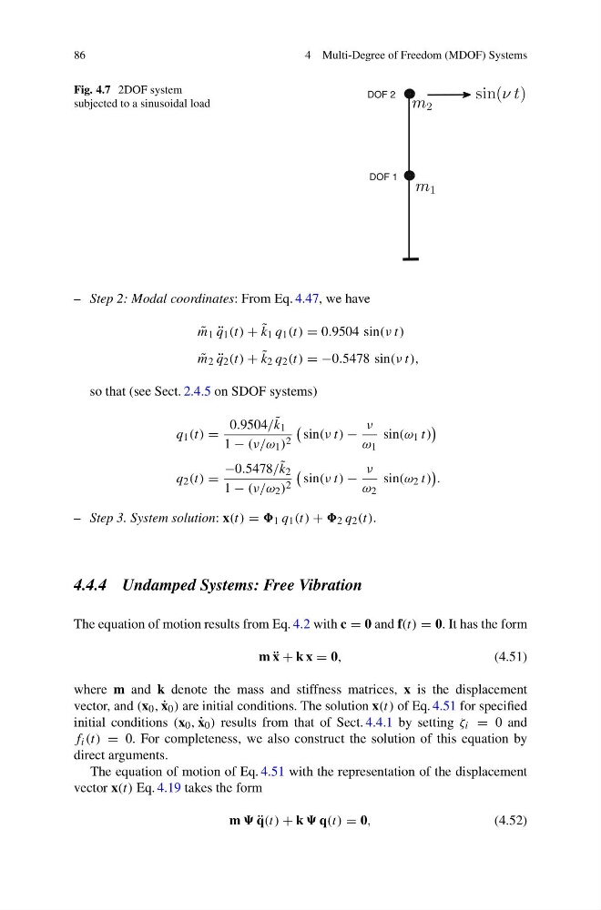
Fig. 4.7 2DOF system
subjected to a sinusoidal load
DOF 2
DOF 1
m 2
m 1
sin(ν t)
– Step 2: Modal coordinates: From Eq. 4.47, we have
˜
m 1 ¨
q 1 (t) + ˜
k 1 q 1 (t) = 0.9504 sin(ν t)
˜
m 2 ¨
q 2 (t) + ˜
k 2 q 2 (t) = −0.5478 sin(ν t),
so that (see Sect. 2.4.5 on SDOF systems)
q 1 (t) =
0.9504/ ˜
k 1
1 − (ν/ω 1 ) 2
sin(ν t) −
ν
ω 1
sin(ω 1 t)
q 2 (t) =
−0.5478/ ˜
k 2
1 − (ν/ω 2 ) 2
sin(ν t) −
ν
ω 2
sin(ω 2 t)
.
– Step 3. System solution: x(t) = 1 q 1 (t) + 2 q 2 (t).
4.4.4 Undamped Systems: Free Vibration
The equation of motion results from Eq. 4.2 with c = 0 and f(t) = 0. It has the form
m ¨
x + k x = 0,
(4.51)
where m and k denote the mass and stiffness matrices, x is the displacement
vector, and (x 0 , ˙
x 0 ) are initial conditions. The solution x(t) of Eq. 4.51 for specified
initial conditions (x 0 , ˙
x 0 ) results from that of Sect. 4.4.1 by setting ζ i = 0 and
f i (t) = 0. For completeness, we also construct the solution of this equation by
direct arguments.
The equation of motion of Eq. 4.51 with the representation of the displacement
vector x(t) Eq. 4.19 takes the form
m ¨
q(t) + k q(t) = 0,
(4.52)
4 Multi-Degree of Freedom (MDOF) Systems
Fig. 4.7 2DOF system
subjected to a sinusoidal load
DOF 2
DOF 1
m 2
m 1
sin(ν t)
– Step 2: Modal coordinates: From Eq. 4.47, we have
˜
m 1 ¨
q 1 (t) + ˜
k 1 q 1 (t) = 0.9504 sin(ν t)
˜
m 2 ¨
q 2 (t) + ˜
k 2 q 2 (t) = −0.5478 sin(ν t),
so that (see Sect. 2.4.5 on SDOF systems)
q 1 (t) =
0.9504/ ˜
k 1
1 − (ν/ω 1 ) 2
sin(ν t) −
ν
ω 1
sin(ω 1 t)
q 2 (t) =
−0.5478/ ˜
k 2
1 − (ν/ω 2 ) 2
sin(ν t) −
ν
ω 2
sin(ω 2 t)
.
– Step 3. System solution: x(t) = 1 q 1 (t) + 2 q 2 (t).
4.4.4 Undamped Systems: Free Vibration
The equation of motion results from Eq. 4.2 with c = 0 and f(t) = 0. It has the form
m ¨
x + k x = 0,
(4.51)
where m and k denote the mass and stiffness matrices, x is the displacement
vector, and (x 0 , ˙
x 0 ) are initial conditions. The solution x(t) of Eq. 4.51 for specified
initial conditions (x 0 , ˙
x 0 ) results from that of Sect. 4.4.1 by setting ζ i = 0 and
f i (t) = 0. For completeness, we also construct the solution of this equation by
direct arguments.
The equation of motion of Eq. 4.51 with the representation of the displacement
vector x(t) Eq. 4.19 takes the form
m ¨
q(t) + k q(t) = 0,
(4.52)