

4.3 Classical Modal Analysis
73
=
n
i=1 b 2
i ω 2
i ˜
m i
n
i=1 b 2
i ˜
m i
=
n
i=1
b 2
i ˜
m i
n
j =1 b 2
j ˜
m j
ω
2
i =
n
i=1
d
2
i ω
2
i ,
where d
2
i =
b 2
i ˜
m i
n
j =1 b 2
j ˜
m j
.
Note that
n
i=1 d 2
i = 1 and that ω 2 given by the above result take values in the
range [ω 2
1 , ω 2
n ] since
ω
2
=
n
i=1
d
2
i ω
2
i ≤
n
i=1
d
2
i ω
2
n = ω
2
n and ω
2
=
n
i=1
d
2
i ω
2
i ≥
n
i=1
d
2
i ω
2
1 = ω
2
1 ,
which proves Eq. 4.12.
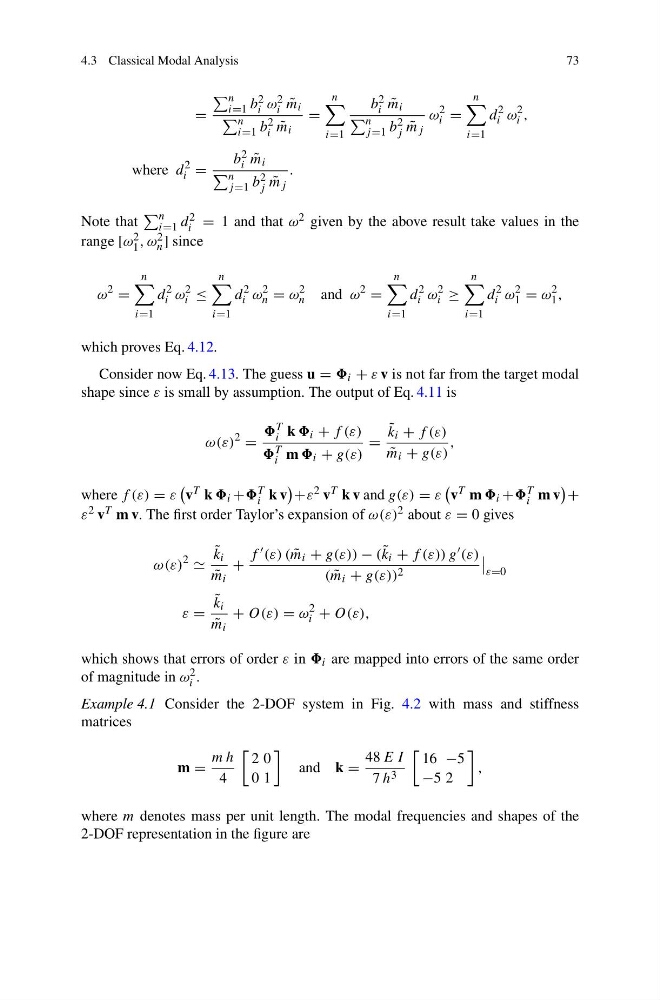
Consider now Eq. 4.13. The guess u = i + ε v is not far from the target modal
shape since ε is small by assumption. The output of Eq. 4.11 is
ω(ε)
2
=
T
i k i + f (ε)
T
i m i + g(ε)
=
˜
k i + f (ε)
˜
m i + g(ε)
,
where f (ε) = ε
v T k i + T
i k v
+ε 2 v T k v and g(ε) = ε
v T m i + T
i m v
+
ε 2 v T m v. The first order Taylor’s expansion of ω(ε) 2 about ε = 0 gives
ω(ε)
2
˜
k i
˜
m i
+
f (ε) ( ˜
m i + g(ε)) − ( ˜
k i + f (ε)) g (ε)
( ˜
m i + g(ε)) 2
ε=0
ε =
˜
k i
˜
m i
+ O(ε) = ω
2
i + O(ε),
which shows that errors of order ε in i are mapped into errors of the same order
of magnitude in ω 2
i .
Example 4.1 Consider the 2-DOF system in Fig. 4.2 with mass and stiffness
matrices
m =
m h
4
2 0
0 1
and k =
48 E I
7 h 3
16 −5
−5 2
,
where m denotes mass per unit length. The modal frequencies and shapes of the
2-DOF representation in the figure are
73
=
n
i=1 b 2
i ω 2
i ˜
m i
n
i=1 b 2
i ˜
m i
=
n
i=1
b 2
i ˜
m i
n
j =1 b 2
j ˜
m j
ω
2
i =
n
i=1
d
2
i ω
2
i ,
where d
2
i =
b 2
i ˜
m i
n
j =1 b 2
j ˜
m j
.
Note that
n
i=1 d 2
i = 1 and that ω 2 given by the above result take values in the
range [ω 2
1 , ω 2
n ] since
ω
2
=
n
i=1
d
2
i ω
2
i ≤
n
i=1
d
2
i ω
2
n = ω
2
n and ω
2
=
n
i=1
d
2
i ω
2
i ≥
n
i=1
d
2
i ω
2
1 = ω
2
1 ,
which proves Eq. 4.12.
Consider now Eq. 4.13. The guess u = i + ε v is not far from the target modal
shape since ε is small by assumption. The output of Eq. 4.11 is
ω(ε)
2
=
T
i k i + f (ε)
T
i m i + g(ε)
=
˜
k i + f (ε)
˜
m i + g(ε)
,
where f (ε) = ε
v T k i + T
i k v
+ε 2 v T k v and g(ε) = ε
v T m i + T
i m v
+
ε 2 v T m v. The first order Taylor’s expansion of ω(ε) 2 about ε = 0 gives
ω(ε)
2
˜
k i
˜
m i
+
f (ε) ( ˜
m i + g(ε)) − ( ˜
k i + f (ε)) g (ε)
( ˜
m i + g(ε)) 2
ε=0
ε =
˜
k i
˜
m i
+ O(ε) = ω
2
i + O(ε),
which shows that errors of order ε in i are mapped into errors of the same order
of magnitude in ω 2
i .
Example 4.1 Consider the 2-DOF system in Fig. 4.2 with mass and stiffness
matrices
m =
m h
4
2 0
0 1
and k =
48 E I
7 h 3
16 −5
−5 2
,
where m denotes mass per unit length. The modal frequencies and shapes of the
2-DOF representation in the figure are