

2.7 Applications
47
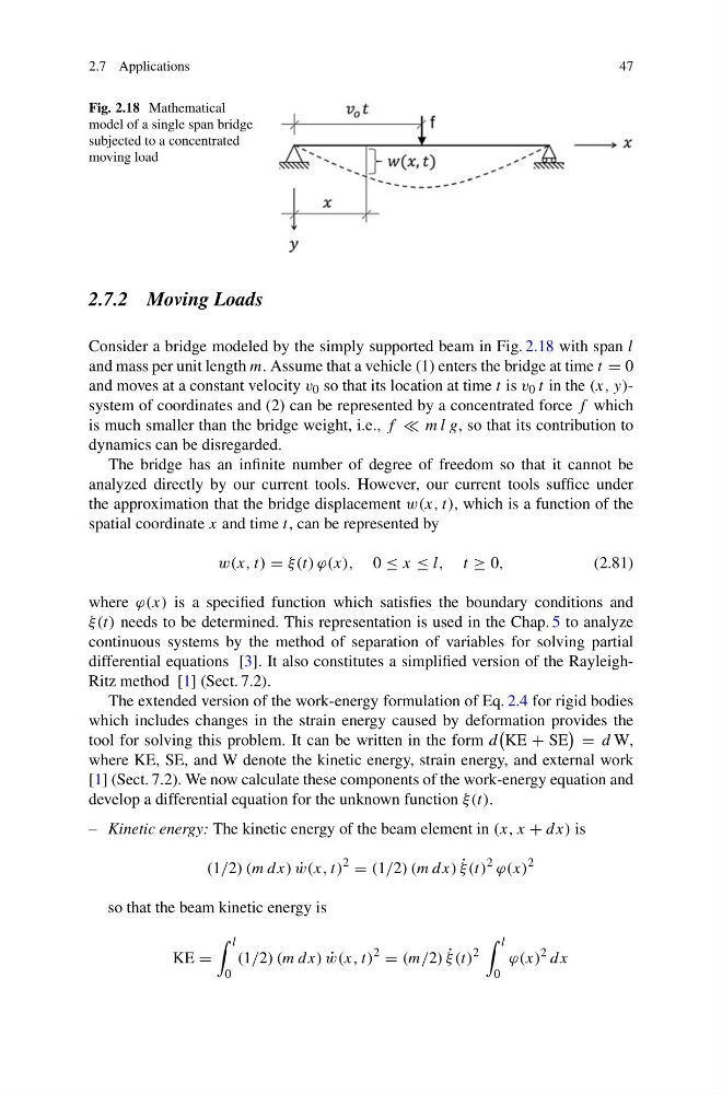
Fig. 2.18 Mathematical
model of a single span bridge
subjected to a concentrated
moving load
2.7.2 Moving Loads
Consider a bridge modeled by the simply supported beam in Fig. 2.18 with span l
and mass per unit length m. Assume that a vehicle (1) enters the bridge at time t = 0
and moves at a constant velocity v 0 so that its location at time t is v 0 t in the (x, y)system of coordinates and (2) can be represented by a concentrated force f which
is much smaller than the bridge weight, i.e., f m l g, so that its contribution to
dynamics can be disregarded.
The bridge has an infinite number of degree of freedom so that it cannot be
analyzed directly by our current tools. However, our current tools suffice under
the approximation that the bridge displacement w(x, t), which is a function of the
spatial coordinate x and time t, can be represented by
w(x, t) = ξ(t) ϕ(x), 0 ≤ x ≤ l, t ≥ 0,
(2.81)
where ϕ(x) is a specified function which satisfies the boundary conditions and
ξ(t) needs to be determined. This representation is used in the Chap. 5 to analyze
continuous systems by the method of separation of variables for solving partial
differential equations [3]. It also constitutes a simplified version of the RayleighRitz method [1] (Sect. 7.2).
The extended version of the work-energy formulation of Eq. 2.4 for rigid bodies
which includes changes in the strain energy caused by deformation provides the
tool for solving this problem. It can be written in the form d
KE + SE
= d W,
where KE, SE, and W denote the kinetic energy, strain energy, and external work
[1] (Sect. 7.2). We now calculate these components of the work-energy equation and
develop a differential equation for the unknown function ξ(t).
– Kinetic energy: The kinetic energy of the beam element in (x, x + dx) is
(1/2) (m dx) ˙
w(x, t)
2
= (1/2) (m dx) ˙
ξ (t)
2 ϕ(x)
2
so that the beam kinetic energy is
KE =
l
0
(1/2) (m dx) ˙
w(x, t)
2
= (m/2) ˙
ξ(t)
2
l
0
ϕ(x)
2 dx
47
Fig. 2.18 Mathematical
model of a single span bridge
subjected to a concentrated
moving load
2.7.2 Moving Loads
Consider a bridge modeled by the simply supported beam in Fig. 2.18 with span l
and mass per unit length m. Assume that a vehicle (1) enters the bridge at time t = 0
and moves at a constant velocity v 0 so that its location at time t is v 0 t in the (x, y)system of coordinates and (2) can be represented by a concentrated force f which
is much smaller than the bridge weight, i.e., f m l g, so that its contribution to
dynamics can be disregarded.
The bridge has an infinite number of degree of freedom so that it cannot be
analyzed directly by our current tools. However, our current tools suffice under
the approximation that the bridge displacement w(x, t), which is a function of the
spatial coordinate x and time t, can be represented by
w(x, t) = ξ(t) ϕ(x), 0 ≤ x ≤ l, t ≥ 0,
(2.81)
where ϕ(x) is a specified function which satisfies the boundary conditions and
ξ(t) needs to be determined. This representation is used in the Chap. 5 to analyze
continuous systems by the method of separation of variables for solving partial
differential equations [3]. It also constitutes a simplified version of the RayleighRitz method [1] (Sect. 7.2).
The extended version of the work-energy formulation of Eq. 2.4 for rigid bodies
which includes changes in the strain energy caused by deformation provides the
tool for solving this problem. It can be written in the form d
KE + SE
= d W,
where KE, SE, and W denote the kinetic energy, strain energy, and external work
[1] (Sect. 7.2). We now calculate these components of the work-energy equation and
develop a differential equation for the unknown function ξ(t).
– Kinetic energy: The kinetic energy of the beam element in (x, x + dx) is
(1/2) (m dx) ˙
w(x, t)
2
= (1/2) (m dx) ˙
ξ (t)
2 ϕ(x)
2
so that the beam kinetic energy is
KE =
l
0
(1/2) (m dx) ˙
w(x, t)
2
= (m/2) ˙
ξ(t)
2
l
0
ϕ(x)
2 dx