

44
2 Single Degree of Freedom (SDOF) Systems
I
c,i (t) =
t
0
∂h(t − u)
∂t
cos(ν i u) du + h(0) cos(ν i t) ⇒ I
c,i (0) = 0 and
I
s,i (t) =
t
0
∂h(t − u)
∂t
sin(ν i u) du + h(0) sin(ν i t) ⇒ I
s,i (0) = 0
since h(0) = 0. Then, the initial conditions x k (0) = x 0 and ˙
x k (0) = ˙
x 0 imply
A k = x 0 and −ζ ω A k + ω d B k = ˙
x 0 , so that
x k (t) = e
−ζ ω t
x 0 cos(ω d t) +
˙
x 0 + ζ ω x 0
ω d
sin(ω d t)
+
n
i=1
a k,i I c,i (t) + b k,i I s,i (t)
.
(2.77)
Since {a k,i }, {b k,i }, {I c,i (t)}, and {I s,i (t)} are known, the time histories of the
displacements {x k (t)}, k = 1, . . . , m, result by elementary calculations.
Example 2.16 Consider an oscillator with natural frequency ω = π , damping ratio
ζ = 0.05, and mass m = 1 which is at rest at the initial time. The system is subjected
to a family of two forcing functions {f k,n (t)}, k = 1, 2, given by Eq. 2.73 with
n = 3, a 1,0 = a 2,0 = 0,
a 1,1 , a 1,2 , a 1,3
= (2, 4, 3),
b 1,1 , b 1,2 , b 1,3
= (1, 2, 3),
a 2,1 , a 2,2 , a 2,3
= (−5, −2, 5) and
b 2,1 , b 2,2 , b 2,3
= (2, 1, 3).
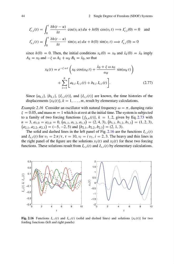
The solid and dashed lines in the left panel of Fig. 2.16 are the functions I c,i (t)
and I s,i (t) for ν 1 = 2 π/τ , τ = 10, ν i = i ν 1 , i = 2, 3. The heavy and thin lines in
the right panel of the figure are the solutions x 1 (t) and x 2 (t) for these two forcing
functions. These solutions result from I c,i (t) and I s,i (t) by elementary calculations.
0
2
4
6
8
10
−0.4
−0.3
−0.2
−0.1
0
0.1
0.2
0.3
t
I
c,i (t) & I
s,i (t)
0
2
4
6
8
10
−2
−1.5
−1
−0.5
0
0.5
1
1.5
2
t
x
k (t)
Fig. 2.16 Functions I c,i (t) and I s,i (t) (solid and dashed lines) and solutions {x k (t)} for two
fording functions (left and right panels)
2 Single Degree of Freedom (SDOF) Systems
I
c,i (t) =
t
0
∂h(t − u)
∂t
cos(ν i u) du + h(0) cos(ν i t) ⇒ I
c,i (0) = 0 and
I
s,i (t) =
t
0
∂h(t − u)
∂t
sin(ν i u) du + h(0) sin(ν i t) ⇒ I
s,i (0) = 0
since h(0) = 0. Then, the initial conditions x k (0) = x 0 and ˙
x k (0) = ˙
x 0 imply
A k = x 0 and −ζ ω A k + ω d B k = ˙
x 0 , so that
x k (t) = e
−ζ ω t
x 0 cos(ω d t) +
˙
x 0 + ζ ω x 0
ω d
sin(ω d t)
+
n
i=1
a k,i I c,i (t) + b k,i I s,i (t)
.
(2.77)
Since {a k,i }, {b k,i }, {I c,i (t)}, and {I s,i (t)} are known, the time histories of the
displacements {x k (t)}, k = 1, . . . , m, result by elementary calculations.
Example 2.16 Consider an oscillator with natural frequency ω = π , damping ratio
ζ = 0.05, and mass m = 1 which is at rest at the initial time. The system is subjected
to a family of two forcing functions {f k,n (t)}, k = 1, 2, given by Eq. 2.73 with
n = 3, a 1,0 = a 2,0 = 0,
a 1,1 , a 1,2 , a 1,3
= (2, 4, 3),
b 1,1 , b 1,2 , b 1,3
= (1, 2, 3),
a 2,1 , a 2,2 , a 2,3
= (−5, −2, 5) and
b 2,1 , b 2,2 , b 2,3
= (2, 1, 3).
The solid and dashed lines in the left panel of Fig. 2.16 are the functions I c,i (t)
and I s,i (t) for ν 1 = 2 π/τ , τ = 10, ν i = i ν 1 , i = 2, 3. The heavy and thin lines in
the right panel of the figure are the solutions x 1 (t) and x 2 (t) for these two forcing
functions. These solutions result from I c,i (t) and I s,i (t) by elementary calculations.
0
2
4
6
8
10
−0.4
−0.3
−0.2
−0.1
0
0.1
0.2
0.3
t
I
c,i (t) & I
s,i (t)
0
2
4
6
8
10
−2
−1.5
−1
−0.5
0
0.5
1
1.5
2
t
x
k (t)
Fig. 2.16 Functions I c,i (t) and I s,i (t) (solid and dashed lines) and solutions {x k (t)} for two
fording functions (left and right panels)