

2.5 Frequency Domain Analysis
35
0
2
4
6
8
10
−2.5
−2
−1.5
−1
−0.5
0
0.5
1
1.5
2
2.5
t
f (t) & f
n (t)
0
2
4
6
8
10
−2.5
−2
−1.5
−1
−0.5
0
0.5
1
1.5
2
2.5
t
f (t) & f
n (t)
0
2
4
6
8
10
−2.5
−2
−1.5
−1
−0.5
0
0.5
1
1.5
2
2.5
t
f (t) & f
n (t)
0
2
4
6
8
10
−2.5
−2
−1.5
−1
−0.5
0
0.5
1
1.5
2
2.5
t
f (t) & f
n (t)
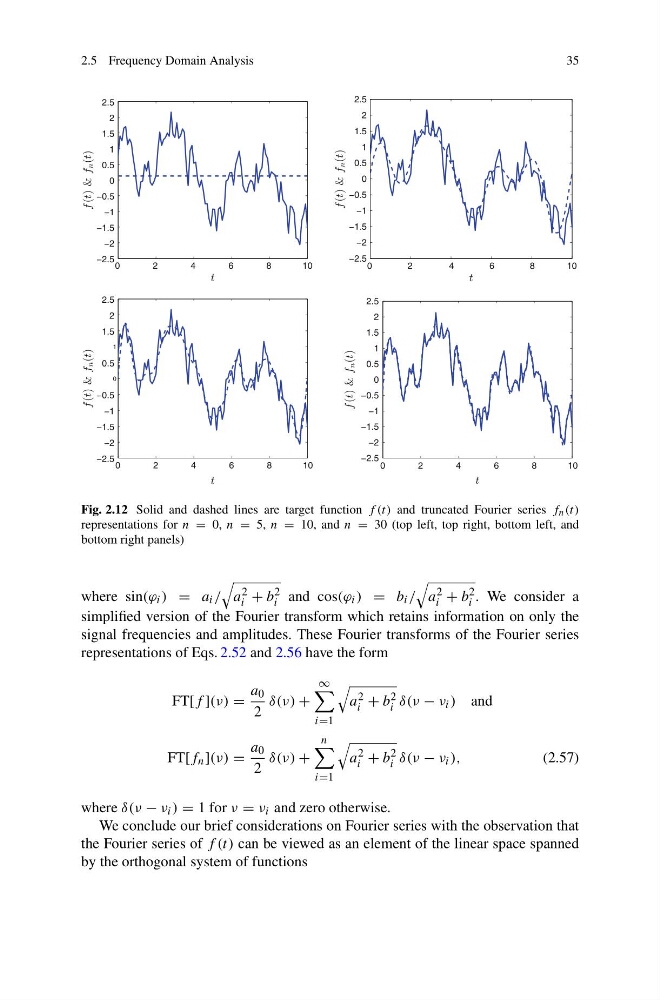
Fig. 2.12 Solid and dashed lines are target function f (t) and truncated Fourier series f n (t)
representations for n = 0, n = 5, n = 10, and n = 30 (top left, top right, bottom left, and
bottom right panels)
where sin(ϕ i ) = a i /
a 2
i + b 2
i and cos(ϕ i ) = b i /
a 2
i + b 2
i . We consider a
simplified version of the Fourier transform which retains information on only the
signal frequencies and amplitudes. These Fourier transforms of the Fourier series
representations of Eqs. 2.52 and 2.56 have the form
FT[f ](ν) =
a 0
2
δ(ν) +
∞
i=1
a 2
i + b 2
i δ(ν − ν i ) and
FT[f n ](ν) =
a 0
2
δ(ν) +
n
i=1
a 2
i + b 2
i δ(ν − ν i ),
(2.57)
where δ(ν − ν i ) = 1 for ν = ν i and zero otherwise.
We conclude our brief considerations on Fourier series with the observation that
the Fourier series of f (t) can be viewed as an element of the linear space spanned
by the orthogonal system of functions
35
0
2
4
6
8
10
−2.5
−2
−1.5
−1
−0.5
0
0.5
1
1.5
2
2.5
t
f (t) & f
n (t)
0
2
4
6
8
10
−2.5
−2
−1.5
−1
−0.5
0
0.5
1
1.5
2
2.5
t
f (t) & f
n (t)
0
2
4
6
8
10
−2.5
−2
−1.5
−1
−0.5
0
0.5
1
1.5
2
2.5
t
f (t) & f
n (t)
0
2
4
6
8
10
−2.5
−2
−1.5
−1
−0.5
0
0.5
1
1.5
2
2.5
t
f (t) & f
n (t)
Fig. 2.12 Solid and dashed lines are target function f (t) and truncated Fourier series f n (t)
representations for n = 0, n = 5, n = 10, and n = 30 (top left, top right, bottom left, and
bottom right panels)
where sin(ϕ i ) = a i /
a 2
i + b 2
i and cos(ϕ i ) = b i /
a 2
i + b 2
i . We consider a
simplified version of the Fourier transform which retains information on only the
signal frequencies and amplitudes. These Fourier transforms of the Fourier series
representations of Eqs. 2.52 and 2.56 have the form
FT[f ](ν) =
a 0
2
δ(ν) +
∞
i=1
a 2
i + b 2
i δ(ν − ν i ) and
FT[f n ](ν) =
a 0
2
δ(ν) +
n
i=1
a 2
i + b 2
i δ(ν − ν i ),
(2.57)
where δ(ν − ν i ) = 1 for ν = ν i and zero otherwise.
We conclude our brief considerations on Fourier series with the observation that
the Fourier series of f (t) can be viewed as an element of the linear space spanned
by the orthogonal system of functions