

32
2 Single Degree of Freedom (SDOF) Systems
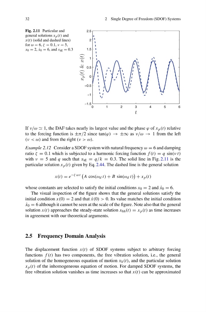
Fig. 2.11 Particular and
general solutions x p (t) and
x(t) (solid and dashed lines)
for ω = 6, ζ = 0.1, ν = 5,
x 0 = 2, ˙
x 0 = 6, and x st = 0.3
0
1
2
3
4
5
6
−1.5
−1
−0.5
0
0.5
1
1.5
2
2.5
t
x
p (t) & x(t)
If ν/ω 1, the DAF takes nearly its largest value and the phase ϕ of x p (t) relative
to the forcing function is ±π/2 since tan(ϕ) → ±∞ as ν/ω → 1 from the left
(ν < ω) and from the right (ν > ω).
Example 2.12 Consider a SDOF system with natural frequency ω = 6 and damping
ratio ζ = 0.1 which is subjected to a harmonic forcing function f (t) = q sin(ν t)
with ν = 5 and q such that x st = q/k = 0.3. The solid line in Fig. 2.11 is the
particular solution x p (t) given by Eq. 2.44. The dashed line is the general solution
x(t) = e
−ζ ω t
A cos(ω d t) + B sin(ω d t)
+ x p (t)
whose constants are selected to satisfy the initial conditions x 0 = 2 and ˙
x 0 = 6.
The visual inspection of the figure shows that the general solutions satisfy the
initial condition x(0) = 2 and that ˙
x(0) > 0. Its value matches the initial condition
˙
x 0 = 6 although it cannot be seen at the scale of the figure. Note also that the general
solution x(t) approaches the steady-state solution x ss (t) = x p (t) as time increases
in agreement with our theoretical arguments.
2.5 Frequency Domain Analysis
The displacement function x(t) of SDOF systems subject to arbitrary forcing
functions f (t) has two components, the free vibration solution, i.e., the general
solution of the homogeneous equation of motion x h (t), and the particular solution
x p (t) of the inhomogeneous equation of motion. For damped SDOF systems, the
free vibration solution vanishes as time increases so that x(t) can be approximated
2 Single Degree of Freedom (SDOF) Systems
Fig. 2.11 Particular and
general solutions x p (t) and
x(t) (solid and dashed lines)
for ω = 6, ζ = 0.1, ν = 5,
x 0 = 2, ˙
x 0 = 6, and x st = 0.3
0
1
2
3
4
5
6
−1.5
−1
−0.5
0
0.5
1
1.5
2
2.5
t
x
p (t) & x(t)
If ν/ω 1, the DAF takes nearly its largest value and the phase ϕ of x p (t) relative
to the forcing function is ±π/2 since tan(ϕ) → ±∞ as ν/ω → 1 from the left
(ν < ω) and from the right (ν > ω).
Example 2.12 Consider a SDOF system with natural frequency ω = 6 and damping
ratio ζ = 0.1 which is subjected to a harmonic forcing function f (t) = q sin(ν t)
with ν = 5 and q such that x st = q/k = 0.3. The solid line in Fig. 2.11 is the
particular solution x p (t) given by Eq. 2.44. The dashed line is the general solution
x(t) = e
−ζ ω t
A cos(ω d t) + B sin(ω d t)
+ x p (t)
whose constants are selected to satisfy the initial conditions x 0 = 2 and ˙
x 0 = 6.
The visual inspection of the figure shows that the general solutions satisfy the
initial condition x(0) = 2 and that ˙
x(0) > 0. Its value matches the initial condition
˙
x 0 = 6 although it cannot be seen at the scale of the figure. Note also that the general
solution x(t) approaches the steady-state solution x ss (t) = x p (t) as time increases
in agreement with our theoretical arguments.
2.5 Frequency Domain Analysis
The displacement function x(t) of SDOF systems subject to arbitrary forcing
functions f (t) has two components, the free vibration solution, i.e., the general
solution of the homogeneous equation of motion x h (t), and the particular solution
x p (t) of the inhomogeneous equation of motion. For damped SDOF systems, the
free vibration solution vanishes as time increases so that x(t) can be approximated