

20
2 Single Degree of Freedom (SDOF) Systems
x(t)=
⎧
⎪ ⎪ ⎪ ⎪ ⎨
⎪ ⎪ ⎪ ⎪ ⎩
0,
for t≤t 1
x st
1 − e −ζ ω (t−t 1 )
cos(ω d (t−t 1 ))+
ζ
√
1−ζ 2
sin(ω d (t−t 1 ))
, for t 1
x((t) cos(ω d (t−t 2 ))+
˙
x((t)+ζ ω x((t)
ω d
sin(ω d (t−t 2 ))
, for t≥t 2 .
(2.28)
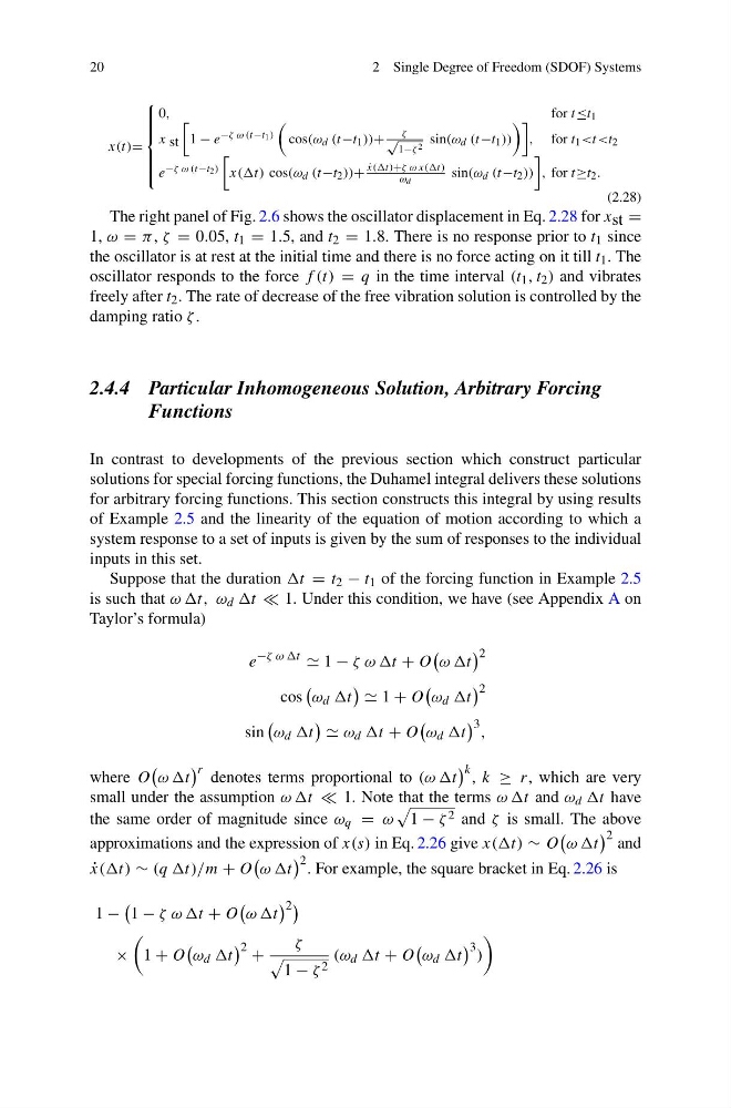
The right panel of Fig. 2.6 shows the oscillator displacement in Eq. 2.28 for x st =
1, ω = π , ζ = 0.05, t 1 = 1.5, and t 2 = 1.8. There is no response prior to t 1 since
the oscillator is at rest at the initial time and there is no force acting on it till t 1 . The
oscillator responds to the force f (t) = q in the time interval (t 1 , t 2 ) and vibrates
freely after t 2 . The rate of decrease of the free vibration solution is controlled by the
damping ratio ζ .
2.4.4 Particular Inhomogeneous Solution, Arbitrary Forcing
Functions
In contrast to developments of the previous section which construct particular
solutions for special forcing functions, the Duhamel integral delivers these solutions
for arbitrary forcing functions. This section constructs this integral by using results
of Example 2.5 and the linearity of the equation of motion according to which a
system response to a set of inputs is given by the sum of responses to the individual
inputs in this set.
Suppose that the duration t = t 2 − t 1 of the forcing function in Example 2.5
is such that ω ωt, ω d t 1. Under this condition, we have (see Appendix A on
Taylor’s formula)
e
−ζ ω ωt
1 − ζ ω ωt + O
ω ωt
2
cos
ω d t
1 + O
ω d t
2
sin
ω d t
ω d t + O
ω d t
3 ,
where O
ω ωt
r denotes terms proportional to (ω ωt
k , k ≥ r, which are very
small under the assumption ω ωt 1. Note that the terms ω ωt and ω d t have
the same order of magnitude since ω q = ω
1 − ζ 2 and ζ is small. The above
approximations and the expression of x(s) in Eq. 2.26 give x(t) ∼ O
ω ωt
2 and
˙
x((t) ∼ (q qt)/m + O
ω ωt
2 . For example, the square bracket in Eq. 2.26 is
1 −
1 − ζ ω ωt + O
ω ωt
2
×
1 + O
ω d t
2 +
ζ
1 − ζ 2
(ω d t + O
ω d t
3 )
2 Single Degree of Freedom (SDOF) Systems
x(t)=
⎧
⎪ ⎪ ⎪ ⎪ ⎨
⎪ ⎪ ⎪ ⎪ ⎩
0,
for t≤t 1
x st
1 − e −ζ ω (t−t 1 )
cos(ω d (t−t 1 ))+
ζ
√
1−ζ 2
sin(ω d (t−t 1 ))
, for t 1
x((t) cos(ω d (t−t 2 ))+
˙
x((t)+ζ ω x((t)
ω d
sin(ω d (t−t 2 ))
, for t≥t 2 .
(2.28)
The right panel of Fig. 2.6 shows the oscillator displacement in Eq. 2.28 for x st =
1, ω = π , ζ = 0.05, t 1 = 1.5, and t 2 = 1.8. There is no response prior to t 1 since
the oscillator is at rest at the initial time and there is no force acting on it till t 1 . The
oscillator responds to the force f (t) = q in the time interval (t 1 , t 2 ) and vibrates
freely after t 2 . The rate of decrease of the free vibration solution is controlled by the
damping ratio ζ .
2.4.4 Particular Inhomogeneous Solution, Arbitrary Forcing
Functions
In contrast to developments of the previous section which construct particular
solutions for special forcing functions, the Duhamel integral delivers these solutions
for arbitrary forcing functions. This section constructs this integral by using results
of Example 2.5 and the linearity of the equation of motion according to which a
system response to a set of inputs is given by the sum of responses to the individual
inputs in this set.
Suppose that the duration t = t 2 − t 1 of the forcing function in Example 2.5
is such that ω ωt, ω d t 1. Under this condition, we have (see Appendix A on
Taylor’s formula)
e
−ζ ω ωt
1 − ζ ω ωt + O
ω ωt
2
cos
ω d t
1 + O
ω d t
2
sin
ω d t
ω d t + O
ω d t
3 ,
where O
ω ωt
r denotes terms proportional to (ω ωt
k , k ≥ r, which are very
small under the assumption ω ωt 1. Note that the terms ω ωt and ω d t have
the same order of magnitude since ω q = ω
1 − ζ 2 and ζ is small. The above
approximations and the expression of x(s) in Eq. 2.26 give x(t) ∼ O
ω ωt
2 and
˙
x((t) ∼ (q qt)/m + O
ω ωt
2 . For example, the square bracket in Eq. 2.26 is
1 −
1 − ζ ω ωt + O
ω ωt
2
×
1 + O
ω d t
2 +
ζ
1 − ζ 2
(ω d t + O
ω d t
3 )