

2.4 Time Domain Analysis
13
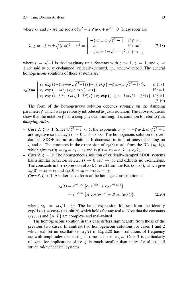
where λ 1 and λ 2 are the roots of λ 2 + 2 ζ ω λ + ω 2 = 0. These roots are
λ 1,2 = −ζ ω ±
(ζ ω) 2 − ω 2 =
⎧
⎪ ⎨
⎪ ⎩
−ζ ω ± ω
ζ 2 − 1, if ζ > 1
−ω,
if ζ = 1
−ζ ω ± i ω
1 − ζ 2 , if ζ < 1,
(2.18)
where i =
√ −1 is the imaginary unit. Systems with ζ > 1, ζ = 1, and ζ <
1 are said to be over-damped, critically-damped, and under-damped. The general
homogeneous solutions of these systems are
x h (t)=
⎧
⎪ ⎨
⎪ ⎩
c 1 exp
(−ζ ω+ω
ζ 2 −1) t
+c 2 exp
(−ζ ω−ω
ζ 2 −1) t
,
if ζ >1
c 1 exp
− ω t
+c 2 t exp
−ω t
,
if ζ =1
c 1 exp
(−ζ ω+i ω
1−ζ 2 ) t
+c 2 exp
(−ζ ω−i ω
1 − ζ 2 ) t
, if ζ <1.
(2.19)
The form of the homogeneous solution depends strongly on the damping
parameter ζ which was previously introduced as just a notation. The above solutions
show that the notation ζ has a deep physical meaning. It is common to refer to ζ as
damping ratio.
– Case 1. ζ > 1: Since
ζ 2 − 1 < ζ, the exponents λ 1,2 = −ζ ω ± ω
ζ 2 − 1
are negative so that x h (t) → 0 as t → ∞. The homogenous solution of overdamped SDOF has no oscillations. It decreases in time at rates depending on
ζ and ω. The constants in the expression of x h (t) result from the ICs (x 0 , ˙
x 0 ),
which give x h (0) = x 0 = c 1 + c 2 and ˙
x h (0) = ˙
x 0 = c 1 λ 1 + c 2 λ 2 .
– Case 2. ζ = 1: The homogeneous solution of critically-damped SDOF systems
has a similar behavior, i.e., x h (t) → 0 as t → ∞ and exhibits no oscillations.
The constants in the expression of x h (t) result from the ICs (x 0 , ˙
x 0 ), which give
x h (0) = x 0 = c 1 and ˙
x h (0) = ˙
x 0 = −c 1 ω + c 2 .
– Case 3. ζ < 1: An alternative form of the homogeneous solution is
x h (t) = e
−ζ ω t
c 1 e
i ω d t
+ c 2 e
−i ω d t
= e
−ζ ω t
A cos(ω d t) + B sin(ω d t)
,
(2.20)
where ω d = ω
1 − ζ 2 . The latter expression follows from the identity
exp(±i u) = cos(u)±i sin(u) which holds for any real u. Note that the constants
c 1 , c 2
and
A, B
are complex- and real-valued.
The homogeneous solution in this case differs significantly from those of the
previous two cases. In contrast two homogeneous solutions for cases 1 and 2
which exhibit no oscillations, x h (t) in Eq. 2.20 has oscillations of frequency
ω d with amplitudes decreasing in time at the rate ζ ω. Case 3 is particularly
relevant for applications since ζ is much smaller than unity for almost all
structural/mechanical systems.
13
where λ 1 and λ 2 are the roots of λ 2 + 2 ζ ω λ + ω 2 = 0. These roots are
λ 1,2 = −ζ ω ±
(ζ ω) 2 − ω 2 =
⎧
⎪ ⎨
⎪ ⎩
−ζ ω ± ω
ζ 2 − 1, if ζ > 1
−ω,
if ζ = 1
−ζ ω ± i ω
1 − ζ 2 , if ζ < 1,
(2.18)
where i =
√ −1 is the imaginary unit. Systems with ζ > 1, ζ = 1, and ζ <
1 are said to be over-damped, critically-damped, and under-damped. The general
homogeneous solutions of these systems are
x h (t)=
⎧
⎪ ⎨
⎪ ⎩
c 1 exp
(−ζ ω+ω
ζ 2 −1) t
+c 2 exp
(−ζ ω−ω
ζ 2 −1) t
,
if ζ >1
c 1 exp
− ω t
+c 2 t exp
−ω t
,
if ζ =1
c 1 exp
(−ζ ω+i ω
1−ζ 2 ) t
+c 2 exp
(−ζ ω−i ω
1 − ζ 2 ) t
, if ζ <1.
(2.19)
The form of the homogeneous solution depends strongly on the damping
parameter ζ which was previously introduced as just a notation. The above solutions
show that the notation ζ has a deep physical meaning. It is common to refer to ζ as
damping ratio.
– Case 1. ζ > 1: Since
ζ 2 − 1 < ζ, the exponents λ 1,2 = −ζ ω ± ω
ζ 2 − 1
are negative so that x h (t) → 0 as t → ∞. The homogenous solution of overdamped SDOF has no oscillations. It decreases in time at rates depending on
ζ and ω. The constants in the expression of x h (t) result from the ICs (x 0 , ˙
x 0 ),
which give x h (0) = x 0 = c 1 + c 2 and ˙
x h (0) = ˙
x 0 = c 1 λ 1 + c 2 λ 2 .
– Case 2. ζ = 1: The homogeneous solution of critically-damped SDOF systems
has a similar behavior, i.e., x h (t) → 0 as t → ∞ and exhibits no oscillations.
The constants in the expression of x h (t) result from the ICs (x 0 , ˙
x 0 ), which give
x h (0) = x 0 = c 1 and ˙
x h (0) = ˙
x 0 = −c 1 ω + c 2 .
– Case 3. ζ < 1: An alternative form of the homogeneous solution is
x h (t) = e
−ζ ω t
c 1 e
i ω d t
+ c 2 e
−i ω d t
= e
−ζ ω t
A cos(ω d t) + B sin(ω d t)
,
(2.20)
where ω d = ω
1 − ζ 2 . The latter expression follows from the identity
exp(±i u) = cos(u)±i sin(u) which holds for any real u. Note that the constants
c 1 , c 2
and
A, B
are complex- and real-valued.
The homogeneous solution in this case differs significantly from those of the
previous two cases. In contrast two homogeneous solutions for cases 1 and 2
which exhibit no oscillations, x h (t) in Eq. 2.20 has oscillations of frequency
ω d with amplitudes decreasing in time at the rate ζ ω. Case 3 is particularly
relevant for applications since ζ is much smaller than unity for almost all
structural/mechanical systems.