

8
2 Single Degree of Freedom (SDOF) Systems
δ = δ st
1 +
1 +
2 h
δ st
> δ st .
(2.6)
Note that δ is twice as large as the statistical deformation δ st if the spring is loaded
suddenly (h = 0) rather than statically.
2.2 Physical System
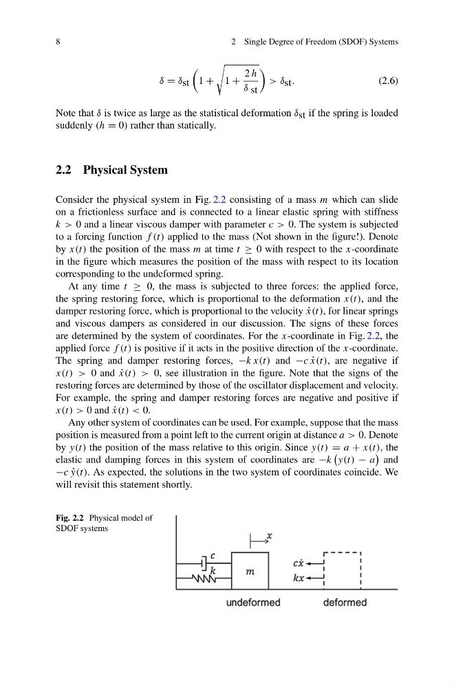
Consider the physical system in Fig. 2.2 consisting of a mass m which can slide
on a frictionless surface and is connected to a linear elastic spring with stiffness
k > 0 and a linear viscous damper with parameter c > 0. The system is subjected
to a forcing function f (t) applied to the mass (Not shown in the figure!). Denote
by x(t) the position of the mass m at time t ≥ 0 with respect to the x-coordinate
in the figure which measures the position of the mass with respect to its location
corresponding to the undeformed spring.
At any time t ≥ 0, the mass is subjected to three forces: the applied force,
the spring restoring force, which is proportional to the deformation x(t), and the
damper restoring force, which is proportional to the velocity ˙
x(t), for linear springs
and viscous dampers as considered in our discussion. The signs of these forces
are determined by the system of coordinates. For the x-coordinate in Fig. 2.2, the
applied force f (t) is positive if it acts in the positive direction of the x-coordinate.
The spring and damper restoring forces, −k x(t) and −c ˙
x(t), are negative if
x(t) > 0 and ˙
x(t) > 0, see illustration in the figure. Note that the signs of the
restoring forces are determined by those of the oscillator displacement and velocity.
For example, the spring and damper restoring forces are negative and positive if
x(t) > 0 and ˙
x(t) < 0.
Any other system of coordinates can be used. For example, suppose that the mass
position is measured from a point left to the current origin at distance a > 0. Denote
by y(t) the position of the mass relative to this origin. Since y(t) = a + x(t), the
elastic and damping forces in this system of coordinates are −k
y(t) − a
and
−c ˙
y(t). As expected, the solutions in the two system of coordinates coincide. We
will revisit this statement shortly.
Fig. 2.2 Physical model of
SDOF systems
2 Single Degree of Freedom (SDOF) Systems
δ = δ st
1 +
1 +
2 h
δ st
> δ st .
(2.6)
Note that δ is twice as large as the statistical deformation δ st if the spring is loaded
suddenly (h = 0) rather than statically.
2.2 Physical System
Consider the physical system in Fig. 2.2 consisting of a mass m which can slide
on a frictionless surface and is connected to a linear elastic spring with stiffness
k > 0 and a linear viscous damper with parameter c > 0. The system is subjected
to a forcing function f (t) applied to the mass (Not shown in the figure!). Denote
by x(t) the position of the mass m at time t ≥ 0 with respect to the x-coordinate
in the figure which measures the position of the mass with respect to its location
corresponding to the undeformed spring.
At any time t ≥ 0, the mass is subjected to three forces: the applied force,
the spring restoring force, which is proportional to the deformation x(t), and the
damper restoring force, which is proportional to the velocity ˙
x(t), for linear springs
and viscous dampers as considered in our discussion. The signs of these forces
are determined by the system of coordinates. For the x-coordinate in Fig. 2.2, the
applied force f (t) is positive if it acts in the positive direction of the x-coordinate.
The spring and damper restoring forces, −k x(t) and −c ˙
x(t), are negative if
x(t) > 0 and ˙
x(t) > 0, see illustration in the figure. Note that the signs of the
restoring forces are determined by those of the oscillator displacement and velocity.
For example, the spring and damper restoring forces are negative and positive if
x(t) > 0 and ˙
x(t) < 0.
Any other system of coordinates can be used. For example, suppose that the mass
position is measured from a point left to the current origin at distance a > 0. Denote
by y(t) the position of the mass relative to this origin. Since y(t) = a + x(t), the
elastic and damping forces in this system of coordinates are −k
y(t) − a
and
−c ˙
y(t). As expected, the solutions in the two system of coordinates coincide. We
will revisit this statement shortly.
Fig. 2.2 Physical model of
SDOF systems