

142
C Linear or Vector Spaces
this system of coordinates, x and y admit the representations
x =
n
k=1
x k i k and y =
n
k=1
y k i k ,
(C.2)
where {x k } and {y k }, k = 1, . . . , n, denote the components of x and y, i.e.,
the projections of these vectors on the unit vectors {i k }. The vector addition and
multiplication by scalar is performed, as previously, component-by-components,
i.e.,
x + y =
n
k=1
x k + y k
i k
α x =
n
k=1
α x k
i k .
(C.3)
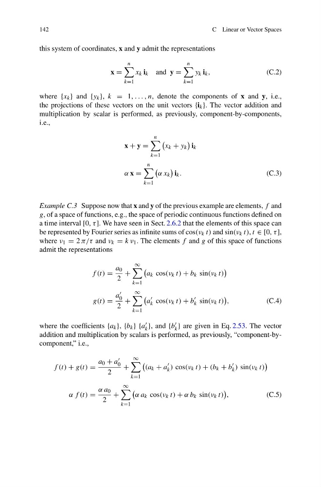
Example C.3 Suppose now that x and y of the previous example are elements, f and
g, of a space of functions, e.g., the space of periodic continuous functions defined on
a time interval [0, τ ]. We have seen in Sect. 2.6.2 that the elements of this space can
be represented by Fourier series as infinite sums of cos(ν k t) and sin(ν k t), t ∈ [0, τ ],
where ν 1 = 2 π/τ and ν k = k ν 1 . The elements f and g of this space of functions
admit the representations
f (t) =
a 0
2
+
∞
k=1
a k cos(ν k t) + b k sin(ν k t)
g(t) =
a
0
2
+
∞
k=1
a
k cos(ν k t) + b
k sin(ν k t)
,
(C.4)
where the coefficients {a k }, {b k } {a
k }, and {b
k } are given in Eq. 2.53. The vector
addition and multiplication by scalars is performed, as previously, “component-bycomponent,” i.e.,
f (t) + g(t) =
a 0 + a
0
2
+
∞
k=1
(a k + a
k ) cos(ν k t) + (b k + b
k ) sin(ν k t)
α f (t) =
α a 0
2
+
∞
k=1
α a k cos(ν k t) + α b k sin(ν k t)
,
(C.5)
C Linear or Vector Spaces
this system of coordinates, x and y admit the representations
x =
n
k=1
x k i k and y =
n
k=1
y k i k ,
(C.2)
where {x k } and {y k }, k = 1, . . . , n, denote the components of x and y, i.e.,
the projections of these vectors on the unit vectors {i k }. The vector addition and
multiplication by scalar is performed, as previously, component-by-components,
i.e.,
x + y =
n
k=1
x k + y k
i k
α x =
n
k=1
α x k
i k .
(C.3)
Example C.3 Suppose now that x and y of the previous example are elements, f and
g, of a space of functions, e.g., the space of periodic continuous functions defined on
a time interval [0, τ ]. We have seen in Sect. 2.6.2 that the elements of this space can
be represented by Fourier series as infinite sums of cos(ν k t) and sin(ν k t), t ∈ [0, τ ],
where ν 1 = 2 π/τ and ν k = k ν 1 . The elements f and g of this space of functions
admit the representations
f (t) =
a 0
2
+
∞
k=1
a k cos(ν k t) + b k sin(ν k t)
g(t) =
a
0
2
+
∞
k=1
a
k cos(ν k t) + b
k sin(ν k t)
,
(C.4)
where the coefficients {a k }, {b k } {a
k }, and {b
k } are given in Eq. 2.53. The vector
addition and multiplication by scalars is performed, as previously, “component-bycomponent,” i.e.,
f (t) + g(t) =
a 0 + a
0
2
+
∞
k=1
(a k + a
k ) cos(ν k t) + (b k + b
k ) sin(ν k t)
α f (t) =
α a 0
2
+
∞
k=1
α a k cos(ν k t) + α b k sin(ν k t)
,
(C.5)