

138
B Linear Differential Equations
The following example deals with a differential equation, which is essential
for the analysis MDOF systems with non-proportional damping. It shows that the
solution of this equation can be obtained by elementary arguments.
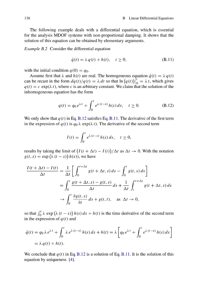
Example B.2 Consider the differential equation
˙
q(t) = λ q(t) + h(t), t ≥ 0,
(B.11)
with the initial condition q(0) = q 0 .
Assume first that λ and h(t) are real. The homogeneous equation ˙
q(t) = λ q(t)
can be recast in the form dq(t)/q(t) = λ dt so that ln
q(t)
t
0
= λ t, which gives
q(t) = c exp(λ t), where c is an arbitrary constant. We claim that the solution of the
inhomogeneous equation has the form
q(t) = q 0 e
λ t
+
t
0
e
λ (t−s) h(s) ds, t ≥ 0.
(B.12)
We only show that q(t) in Eq. B.12 satisfies Eq. B.11. The derivative of the first term
in the expression of q(t) is q 0 λ exp(λ t). The derivative of the second term
I (t) =
t
0
e
λ (t−s) h(s) ds, t ≥ 0,
results by taking the limit of
I (t + − I (t)
//t as t → 0. With the notation
g(t, s) = exp
λ (t − s)
h(s)), we have
I (t + − I (t)
t
=
1
t
t+t
0
g(t + t, s) ds −
t
0
g(t, s) ds
=
t
0
g(t + t, s) − g(t, s)
t
ds +
1
t
t+t
t
g(t + t, s) ds
→
t
0
∂g(t, s)
∂t
ds + g(t, t), as t → 0,
so that
t
0 λ exp
λ (t − s)
h(s) ds + h(t) is the time derivative of the second term
in the expression of q(t) and
˙
q(t) = q 0 λ e
λ t
+
t
0
λ e
λ (t−s) h(s) ds + h(t) = λ
q 0 e
λ t
+
t
0
e
λ (t−s) h(s) ds
= λ q(t) + h(t).
We conclude that q(t) in Eq. B.12 is a solution of Eq. B.11. It is the solution of this
equation by uniqueness [4].
B Linear Differential Equations
The following example deals with a differential equation, which is essential
for the analysis MDOF systems with non-proportional damping. It shows that the
solution of this equation can be obtained by elementary arguments.
Example B.2 Consider the differential equation
˙
q(t) = λ q(t) + h(t), t ≥ 0,
(B.11)
with the initial condition q(0) = q 0 .
Assume first that λ and h(t) are real. The homogeneous equation ˙
q(t) = λ q(t)
can be recast in the form dq(t)/q(t) = λ dt so that ln
q(t)
t
0
= λ t, which gives
q(t) = c exp(λ t), where c is an arbitrary constant. We claim that the solution of the
inhomogeneous equation has the form
q(t) = q 0 e
λ t
+
t
0
e
λ (t−s) h(s) ds, t ≥ 0.
(B.12)
We only show that q(t) in Eq. B.12 satisfies Eq. B.11. The derivative of the first term
in the expression of q(t) is q 0 λ exp(λ t). The derivative of the second term
I (t) =
t
0
e
λ (t−s) h(s) ds, t ≥ 0,
results by taking the limit of
I (t + − I (t)
//t as t → 0. With the notation
g(t, s) = exp
λ (t − s)
h(s)), we have
I (t + − I (t)
t
=
1
t
t+t
0
g(t + t, s) ds −
t
0
g(t, s) ds
=
t
0
g(t + t, s) − g(t, s)
t
ds +
1
t
t+t
t
g(t + t, s) ds
→
t
0
∂g(t, s)
∂t
ds + g(t, t), as t → 0,
so that
t
0 λ exp
λ (t − s)
h(s) ds + h(t) is the time derivative of the second term
in the expression of q(t) and
˙
q(t) = q 0 λ e
λ t
+
t
0
λ e
λ (t−s) h(s) ds + h(t) = λ
q 0 e
λ t
+
t
0
e
λ (t−s) h(s) ds
= λ q(t) + h(t).
We conclude that q(t) in Eq. B.12 is a solution of Eq. B.11. It is the solution of this
equation by uniqueness [4].