

110
4 Multi-Degree of Freedom (MDOF) Systems
˜
z ss (t)
2 n
i=1
u i
t
0
e
λ i (t−s)
α i,0 +
m
j =1
α i,j cos(ν j s) + β i,j sin(ν j s)
ds
=
2 n
i=1
u i
α i,0
t
0
e
λ i (t−s) ds
+
m
j =1
α i,j
t
0
e
λ i (t−s) cos(ν j s) ds + β i,j
t
0
e
λ i (t−s) sin(ν j s) ds
.
(4.108)
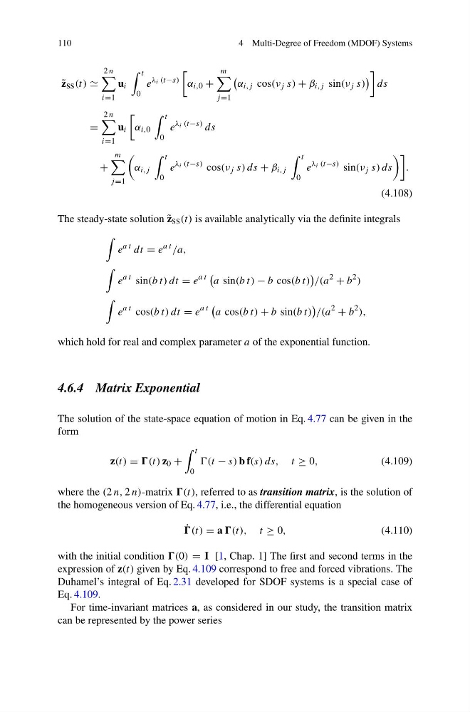
The steady-state solution ˜
z ss (t) is available analytically via the definite integrals
e
a t dt = e
a t /a,
e
a t sin(b t) dt = e
a t
a sin(b t) − b cos(b t)
/(a
2
+ b
2 )
e
a t cos(b t) dt = e
a t
a cos(b t) + b sin(b t)
/(a
2
+ b
2 ),
which hold for real and complex parameter a of the exponential function.
4.6.4 Matrix Exponential
The solution of the state-space equation of motion in Eq. 4.77 can be given in the
form
z(t) = (t) z 0 +
t
0
− s) b f(s) ds, t ≥ 0,
(4.109)
where the (2 n, 2 n)-matrix (t), referred to as transition matrix, is the solution of
the homogeneous version of Eq. 4.77, i.e., the differential equation
˙
(t) = a (t), t ≥ 0,
(4.110)
with the initial condition (0) = I [1, Chap. 1] The first and second terms in the
expression of z(t) given by Eq. 4.109 correspond to free and forced vibrations. The
Duhamel’s integral of Eq. 2.31 developed for SDOF systems is a special case of
Eq. 4.109.
For time-invariant matrices a, as considered in our study, the transition matrix
can be represented by the power series
4 Multi-Degree of Freedom (MDOF) Systems
˜
z ss (t)
2 n
i=1
u i
t
0
e
λ i (t−s)
α i,0 +
m
j =1
α i,j cos(ν j s) + β i,j sin(ν j s)
ds
=
2 n
i=1
u i
α i,0
t
0
e
λ i (t−s) ds
+
m
j =1
α i,j
t
0
e
λ i (t−s) cos(ν j s) ds + β i,j
t
0
e
λ i (t−s) sin(ν j s) ds
.
(4.108)
The steady-state solution ˜
z ss (t) is available analytically via the definite integrals
e
a t dt = e
a t /a,
e
a t sin(b t) dt = e
a t
a sin(b t) − b cos(b t)
/(a
2
+ b
2 )
e
a t cos(b t) dt = e
a t
a cos(b t) + b sin(b t)
/(a
2
+ b
2 ),
which hold for real and complex parameter a of the exponential function.
4.6.4 Matrix Exponential
The solution of the state-space equation of motion in Eq. 4.77 can be given in the
form
z(t) = (t) z 0 +
t
0
− s) b f(s) ds, t ≥ 0,
(4.109)
where the (2 n, 2 n)-matrix (t), referred to as transition matrix, is the solution of
the homogeneous version of Eq. 4.77, i.e., the differential equation
˙
(t) = a (t), t ≥ 0,
(4.110)
with the initial condition (0) = I [1, Chap. 1] The first and second terms in the
expression of z(t) given by Eq. 4.109 correspond to free and forced vibrations. The
Duhamel’s integral of Eq. 2.31 developed for SDOF systems is a special case of
Eq. 4.109.
For time-invariant matrices a, as considered in our study, the transition matrix
can be represented by the power series