

78
S. Goto and H. Hino
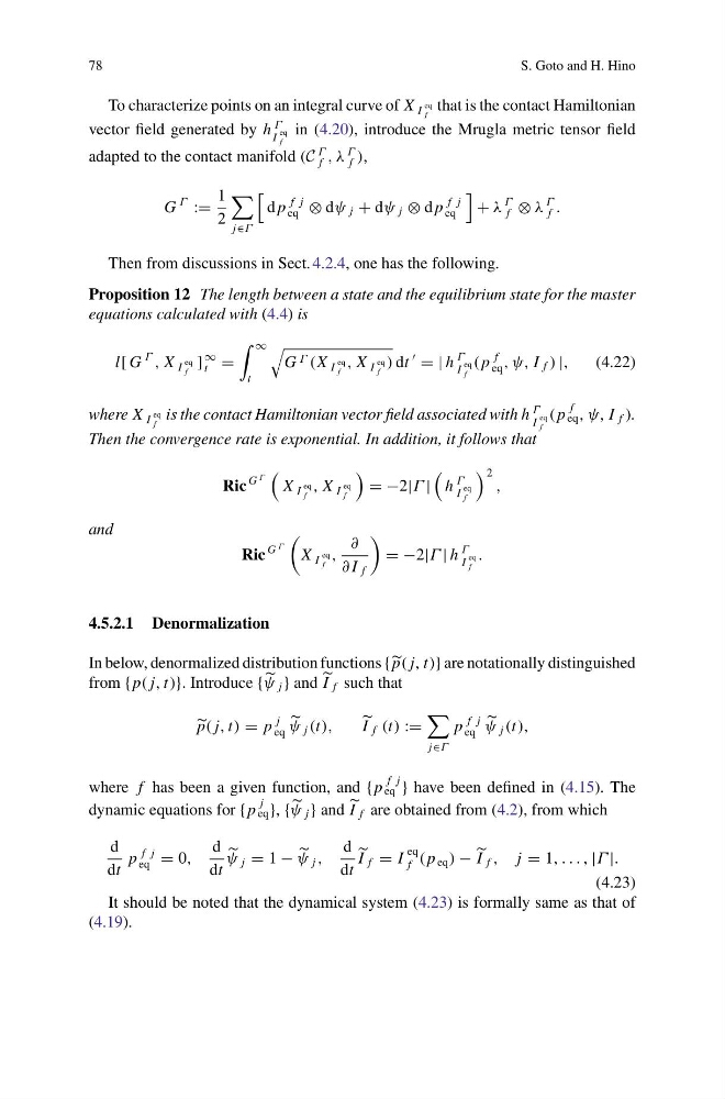
To characterize points on an integral curve of X I
eq
f
that is the contact Hamiltonian
vector field generated by h
Γ
I
eq
f
in (4.20), introduce the Mrugla metric tensor field
adapted to the contact manifold (C
Γ
f , λ
Γ
f ),
G
Γ
:=
1
2
j∈Γ
d p
f j
eq ⊗ dψ j + dψ j ⊗ d p
f j
eq
+ λ
Γ
f ⊗ λ
Γ
f .
Then from discussions in Sect. 4.2.4, one has the following.
Proposition 12 The length between a state and the equilibrium state for the master
equations calculated with (4.4) is
l[ G
Γ
, X I
eq
f
]
∞
t =
∞
t
G Γ (X I
eq
f
, X I
eq
f
) dt
= | h
Γ
I
eq
f
( p
f
eq , ψ, I f ) |,
(4.22)
where X I
eq
f
is the contact Hamiltonian vector field associated with h
Γ
I
eq
f
( p
f
eq , ψ, I f ).
Then the convergence rate is exponential. In addition, it follows that
Ric
G
Γ
X I
eq
f
, X I
eq
f
= −2|Γ |
h
Γ
I
eq
f
2 ,
and
Ric
G
Γ
X I
eq
f
,
∂
∂ I f
= −2|Γ | h
Γ
I
eq
f
.
4.5.2.1 Denormalization
In below, denormalized distribution functions { p( j, t)} are notationally distinguished
from { p( j, t)}. Introduce {
ψ j } and I f such that
p( j, t) = p
j
eq
ψ j (t),
I f (t) :=
j∈Γ
p
f j
eq
ψ j (t),
where f has been a given function, and { p
f j
eq } have been defined in (4.15). The
dynamic equations for { p
j
eq }, {
ψ j } and I f are obtained from (4.2), from which
d
dt
p
f j
eq = 0,
d
dt
ψ j = 1 −
ψ j ,
d
dt
I f = I
eq
f ( p eq ) − I f , j = 1, . . . , |Γ |.
(4.23)
It should be noted that the dynamical system (4.23) is formally same as that of
(4.19).
S. Goto and H. Hino
To characterize points on an integral curve of X I
eq
f
that is the contact Hamiltonian
vector field generated by h
Γ
I
eq
f
in (4.20), introduce the Mrugla metric tensor field
adapted to the contact manifold (C
Γ
f , λ
Γ
f ),
G
Γ
:=
1
2
j∈Γ
d p
f j
eq ⊗ dψ j + dψ j ⊗ d p
f j
eq
+ λ
Γ
f ⊗ λ
Γ
f .
Then from discussions in Sect. 4.2.4, one has the following.
Proposition 12 The length between a state and the equilibrium state for the master
equations calculated with (4.4) is
l[ G
Γ
, X I
eq
f
]
∞
t =
∞
t
G Γ (X I
eq
f
, X I
eq
f
) dt
= | h
Γ
I
eq
f
( p
f
eq , ψ, I f ) |,
(4.22)
where X I
eq
f
is the contact Hamiltonian vector field associated with h
Γ
I
eq
f
( p
f
eq , ψ, I f ).
Then the convergence rate is exponential. In addition, it follows that
Ric
G
Γ
X I
eq
f
, X I
eq
f
= −2|Γ |
h
Γ
I
eq
f
2 ,
and
Ric
G
Γ
X I
eq
f
,
∂
∂ I f
= −2|Γ | h
Γ
I
eq
f
.
4.5.2.1 Denormalization
In below, denormalized distribution functions { p( j, t)} are notationally distinguished
from { p( j, t)}. Introduce {
ψ j } and I f such that
p( j, t) = p
j
eq
ψ j (t),
I f (t) :=
j∈Γ
p
f j
eq
ψ j (t),
where f has been a given function, and { p
f j
eq } have been defined in (4.15). The
dynamic equations for { p
j
eq }, {
ψ j } and I f are obtained from (4.2), from which
d
dt
p
f j
eq = 0,
d
dt
ψ j = 1 −
ψ j ,
d
dt
I f = I
eq
f ( p eq ) − I f , j = 1, . . . , |Γ |.
(4.23)
It should be noted that the dynamical system (4.23) is formally same as that of
(4.19).