

9 Towards the “Shape” of Cosmological Observables and the String …
237
and the vacuum equation is
D φ W = Aφ + B = 0
(9.26)
which is solved by
φ = −
B
A
(9.27)
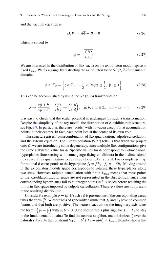
We are interested in the distribution of flux vacua on the axiodilaton moduli space at
fixed L max . We fix a gauge by restricting the axiodilaton to the SL(2, Z) fundamental
domain:
φ ∈ F D =
z ∈ C + : −
1
2
< Re(z) ≤
1
2
, |z| ≥ 1
(9.28)
This can be accomplished by using the SL(2, Z) transformation
φ →
aφ + b
cφ + d
,
f
h
→
a b
c d
, a, b, c, d ∈ Z, ad − bc = 1
(9.29)
It is easy to check that the scalar potential is unchanged by such a transformation.
Despite the simplicity of the toy model, the distribution of φ exhibits rich structure,
see Fig. 9.7. In particular, there are “voids” with no vacua except for at accumulation
points in their centers. In fact, each point lies at the center of its own void.
This structure arises from a combination of flux quantization, tadpole cancellation,
and the F-term equation. The F-term equation (9.27) tells us that when we project
onto φ, we are introducing some degeneracy, since multiple flux configurations give
the same stabilized value for φ. Specific values for φ correspond to 2-dimensional
hyperplanes (intersecting with some gauge-fixing conditions) in the 4-dimensional
flux space. Flux quantization forces these slopes to be rational. For example, φ = iβ
for rational β corresponds to the hyperplane f 1 = βh 2 , f 2 = −βh 1 . Moving around
in the axiodilaton moduli space corresponds to rotating these hyperplanes along
two axes. However, tadpole cancellation with finite L max means that most points
in the axiodilaton moduli space are not represented in the distribution, since their
corresponding hyperplanes fail to hit integer points in flux space before reaching the
limits in flux space imposed by tadpole cancellation. These φ values are not present
in the resulting distribution.
Consider for example φ = iβ. If such a φ is present one of the corresponding vacua
takes the form
i f 1
h 2
. Without loss of generality assume that f 1 and h 2 have no common
factors and that both are positive. The nearest vacuum on the imaginary axis takes
the form i
f 1
h 2
−
a
b
with a, b > 0. (One should use a plus sign for f 1 = h 2 to stay
in the fundamental domain.) To find the nearest neighbor, one minimizes
a
b
over the
naturals subject to the constraint N flux = b
2 f 1 h 2 − abh
2
2 ≤ L max . It can be shown that
237
and the vacuum equation is
D φ W = Aφ + B = 0
(9.26)
which is solved by
φ = −
B
A
(9.27)
We are interested in the distribution of flux vacua on the axiodilaton moduli space at
fixed L max . We fix a gauge by restricting the axiodilaton to the SL(2, Z) fundamental
domain:
φ ∈ F D =
z ∈ C + : −
1
2
< Re(z) ≤
1
2
, |z| ≥ 1
(9.28)
This can be accomplished by using the SL(2, Z) transformation
φ →
aφ + b
cφ + d
,
f
h
→
a b
c d
, a, b, c, d ∈ Z, ad − bc = 1
(9.29)
It is easy to check that the scalar potential is unchanged by such a transformation.
Despite the simplicity of the toy model, the distribution of φ exhibits rich structure,
see Fig. 9.7. In particular, there are “voids” with no vacua except for at accumulation
points in their centers. In fact, each point lies at the center of its own void.
This structure arises from a combination of flux quantization, tadpole cancellation,
and the F-term equation. The F-term equation (9.27) tells us that when we project
onto φ, we are introducing some degeneracy, since multiple flux configurations give
the same stabilized value for φ. Specific values for φ correspond to 2-dimensional
hyperplanes (intersecting with some gauge-fixing conditions) in the 4-dimensional
flux space. Flux quantization forces these slopes to be rational. For example, φ = iβ
for rational β corresponds to the hyperplane f 1 = βh 2 , f 2 = −βh 1 . Moving around
in the axiodilaton moduli space corresponds to rotating these hyperplanes along
two axes. However, tadpole cancellation with finite L max means that most points
in the axiodilaton moduli space are not represented in the distribution, since their
corresponding hyperplanes fail to hit integer points in flux space before reaching the
limits in flux space imposed by tadpole cancellation. These φ values are not present
in the resulting distribution.
Consider for example φ = iβ. If such a φ is present one of the corresponding vacua
takes the form
i f 1
h 2
. Without loss of generality assume that f 1 and h 2 have no common
factors and that both are positive. The nearest vacuum on the imaginary axis takes
the form i
f 1
h 2
−
a
b
with a, b > 0. (One should use a plus sign for f 1 = h 2 to stay
in the fundamental domain.) To find the nearest neighbor, one minimizes
a
b
over the
naturals subject to the constraint N flux = b
2 f 1 h 2 − abh
2
2 ≤ L max . It can be shown that