

9 Towards the “Shape” of Cosmological Observables and the String …
229
dominated by observational effects [5]. We must therefore employ complementary
approaches to data analysis. Current approaches to measuring non-Gaussianity fall
into two categories. The geometric approach aims to quantify the structure of a cosmological observable in position-space. Another approach, which generally takes
place in momentum-space, fits higher-order correlation functions against templates
for different well-motivated models [9, 71].
In this section we review aspects of the geometric approach, focusing on recent
developments and going into more detail regarding the present authors’ contributions.
9.3.1 Morphology of Cosmological Observables: Recent
Progress
Roughly speaking, there are two ways one can gather geometric information from
cosmological observables. The primordial perturbations set up by inflation are naturally described in the language of random fields. For “field-like” observables, one
can consider geometric aspects of excursion sets of the field. For example, primordial
perturbations are imprinted on the Cosmic Microwave Background as temperature
and polarization anisotropies. In the language of Sect. 9.2 one regards e.g.. the temperature anisotropy as a Morse function on the sphere,
ΔT
T avg
: S
2
→ R. Geometric
aspects of the sublevel sets
ΔT
T avg
−1 (−∞, ν] with varying ν are then studied.
On the other hand, we do not observe the density perturbation directly as an
instance of a random field. Rather, we observe tracers of the underlying distribution,
such as galaxies. The organization of this distribution into an intricate hierarchical
network of interlocking filaments, voids, and clusters is sometimes called the cosmic
web [13, 68]. In this context, it is more natural to take a “point-like” viewpoint. As
we saw in Sect. 9.2, persistent homology naturally applies to both contexts.
4
One class of geometric observables in the “field-like” category are the Minkowski
Functionals (MFs) [76, 90, 91, 102]. Analytic expressions for the MFs are known
in the weakly non-Gaussian case [48, 61, 75]. In particular, for the CMB, there are
three MFs: area, length, and “genus” of excursion sets.
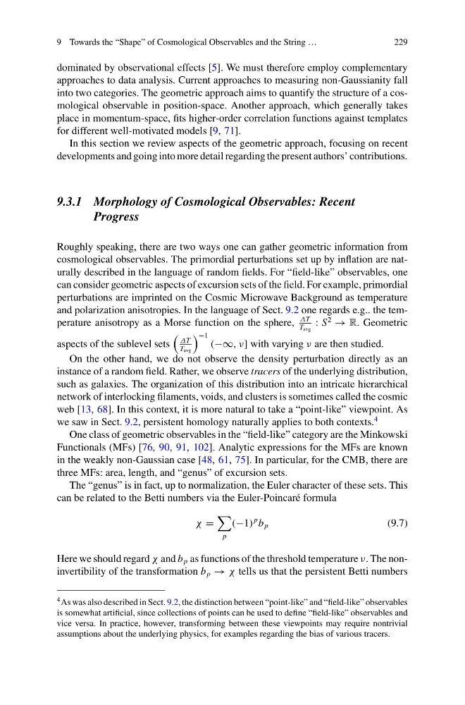
The “genus” is in fact, up to normalization, the Euler character of these sets. This
can be related to the Betti numbers via the Euler-Poincaré formula
χ =
p
(−1)
p b p
(9.7)
Here we should regard χ and b p as functions of the threshold temperature ν. The noninvertibility of the transformation b p → χ tells us that the persistent Betti numbers
4 As was also described in Sect. 9.2, the distinction between “point-like” and “field-like” observables
is somewhat artificial, since collections of points can be used to define “field-like” observables and
vice versa. In practice, however, transforming between these viewpoints may require nontrivial
assumptions about the underlying physics, for examples regarding the bias of various tracers.
229
dominated by observational effects [5]. We must therefore employ complementary
approaches to data analysis. Current approaches to measuring non-Gaussianity fall
into two categories. The geometric approach aims to quantify the structure of a cosmological observable in position-space. Another approach, which generally takes
place in momentum-space, fits higher-order correlation functions against templates
for different well-motivated models [9, 71].
In this section we review aspects of the geometric approach, focusing on recent
developments and going into more detail regarding the present authors’ contributions.
9.3.1 Morphology of Cosmological Observables: Recent
Progress
Roughly speaking, there are two ways one can gather geometric information from
cosmological observables. The primordial perturbations set up by inflation are naturally described in the language of random fields. For “field-like” observables, one
can consider geometric aspects of excursion sets of the field. For example, primordial
perturbations are imprinted on the Cosmic Microwave Background as temperature
and polarization anisotropies. In the language of Sect. 9.2 one regards e.g.. the temperature anisotropy as a Morse function on the sphere,
ΔT
T avg
: S
2
→ R. Geometric
aspects of the sublevel sets
ΔT
T avg
−1 (−∞, ν] with varying ν are then studied.
On the other hand, we do not observe the density perturbation directly as an
instance of a random field. Rather, we observe tracers of the underlying distribution,
such as galaxies. The organization of this distribution into an intricate hierarchical
network of interlocking filaments, voids, and clusters is sometimes called the cosmic
web [13, 68]. In this context, it is more natural to take a “point-like” viewpoint. As
we saw in Sect. 9.2, persistent homology naturally applies to both contexts.
4
One class of geometric observables in the “field-like” category are the Minkowski
Functionals (MFs) [76, 90, 91, 102]. Analytic expressions for the MFs are known
in the weakly non-Gaussian case [48, 61, 75]. In particular, for the CMB, there are
three MFs: area, length, and “genus” of excursion sets.
The “genus” is in fact, up to normalization, the Euler character of these sets. This
can be related to the Betti numbers via the Euler-Poincaré formula
χ =
p
(−1)
p b p
(9.7)
Here we should regard χ and b p as functions of the threshold temperature ν. The noninvertibility of the transformation b p → χ tells us that the persistent Betti numbers
4 As was also described in Sect. 9.2, the distinction between “point-like” and “field-like” observables
is somewhat artificial, since collections of points can be used to define “field-like” observables and
vice versa. In practice, however, transforming between these viewpoints may require nontrivial
assumptions about the underlying physics, for examples regarding the bias of various tracers.