

8 Chain Rule Optimal Transport
209
B. Proof of Upper Bound of H D
Without loss of generality we assume p and q are mixture models. The proof for the
general case is similar.
Proof
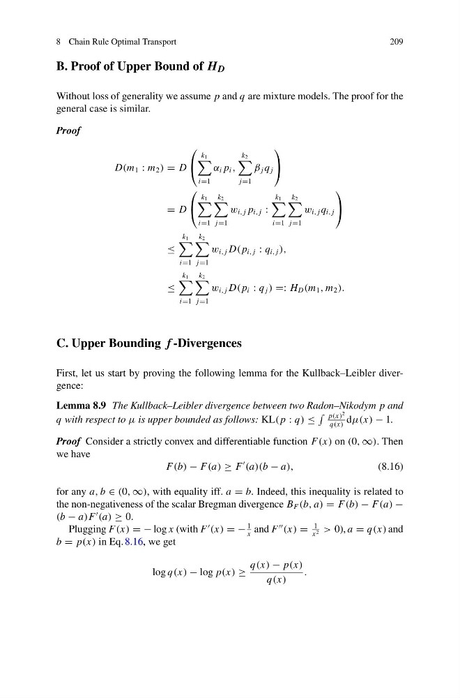
D(m 1 : m 2 ) = D
⎛
⎝
k 1
i=1
α i p i ,
k 2
j=1
β j q j
⎞
⎠
= D
⎛
⎝
k 1
i=1
k 2
j=1
w i, j p i, j :
k 1
i=1
k 2
j=1
w i, j q i, j
⎞
⎠
≤
k 1
i=1
k 2
j=1
w i, j D( p i, j : q i, j ),
≤
k 1
i=1
k 2
j=1
w i, j D( p i : q j ) =: H D (m 1 , m 2 ).
C. Upper Bounding f -Divergences
First, let us start by proving the following lemma for the Kullback–Leibler divergence:
Lemma 8.9 The Kullback–Leibler divergence between two Radon–Nikodym p and
q with respect to μ is upper bounded as follows: KL( p : q) ≤
p(x)
2
q(x)
dμ(x) − 1.
Proof Consider a strictly convex and differentiable function F(x) on (0, ∞). Then
we have
F(b) − F(a) ≥ F
(a)(b − a),
(8.16)
for any a, b ∈ (0, ∞), with equality iff. a = b. Indeed, this inequality is related to
the non-negativeness of the scalar Bregman divergence B F (b, a) = F(b) − F(a) −
(b − a)F
(a) ≥ 0.
Plugging F(x) = − log x (with F
(x) = −
1
x
and F
(x) =
1
x 2 > 0), a = q(x) and
b = p(x) in Eq. 8.16, we get
log q(x) − log p(x) ≥
q(x) − p(x)
q(x)
.
209
B. Proof of Upper Bound of H D
Without loss of generality we assume p and q are mixture models. The proof for the
general case is similar.
Proof
D(m 1 : m 2 ) = D
⎛
⎝
k 1
i=1
α i p i ,
k 2
j=1
β j q j
⎞
⎠
= D
⎛
⎝
k 1
i=1
k 2
j=1
w i, j p i, j :
k 1
i=1
k 2
j=1
w i, j q i, j
⎞
⎠
≤
k 1
i=1
k 2
j=1
w i, j D( p i, j : q i, j ),
≤
k 1
i=1
k 2
j=1
w i, j D( p i : q j ) =: H D (m 1 , m 2 ).
C. Upper Bounding f -Divergences
First, let us start by proving the following lemma for the Kullback–Leibler divergence:
Lemma 8.9 The Kullback–Leibler divergence between two Radon–Nikodym p and
q with respect to μ is upper bounded as follows: KL( p : q) ≤
p(x)
2
q(x)
dμ(x) − 1.
Proof Consider a strictly convex and differentiable function F(x) on (0, ∞). Then
we have
F(b) − F(a) ≥ F
(a)(b − a),
(8.16)
for any a, b ∈ (0, ∞), with equality iff. a = b. Indeed, this inequality is related to
the non-negativeness of the scalar Bregman divergence B F (b, a) = F(b) − F(a) −
(b − a)F
(a) ≥ 0.
Plugging F(x) = − log x (with F
(x) = −
1
x
and F
(x) =
1
x 2 > 0), a = q(x) and
b = p(x) in Eq. 8.16, we get
log q(x) − log p(x) ≥
q(x) − p(x)
q(x)
.